Open PDF
Download PDF
Formulas →
Back to SD-GCM
About this tutorial: This tutorial covers every tab, window, and control in SD-GCM V2.1.
It is written for users who are comfortable with software in general but
new to this specific tool.
Follow the sections in order for a complete first-time walkthrough,
or jump to any section for reference.
SD-GCM V2.1 introduces three new bias-correction methods (QDM, DQM,
SDM), Monthly Stratification, LOCI pre-processing, and a Copernicus CDS
downloader compared to V2.0.
1. Software Overview
SD-GCM (Statistical Downscaling — General Circulation Model) is a
desktop tool for climate scientists, hydrologists, and engineers who
need to bring raw GCM output down to the local scale of observed weather
stations. The core problem it solves: GCMs simulate the global climate
on a coarse grid (typically 50–300 km), but impact studies (flood
modelling, crop simulation, water resource planning) need station-scale
data. SD-GCM applies statistical transfer functions that learn the
relationship between GCM output and observed station data during a
historical calibration period, then apply that relationship to the
future GCM projection to produce a bias-corrected, downscaled time
series.
1.1 The Typical Workflow
Load your observed station data (Station Data tab) — daily,
monthly, or 3-hourly time series from one or more weather
stations.
Load GCM data (Gridded Data tab) — a historical GCM run and a
future SSP/RCP scenario run, either as NetCDF files, Excel/CSV, or
downloaded live from Copernicus CDS.
Evaluate methods (Evaluation tab) — split the historical period
into calibration and evaluation sub-periods, apply each method, and
compare performance metrics to identify the best approach for your
data.
Apply bias correction to the full future period (Bias Correction
tab) — run the chosen method on the future GCM scenario to produce the
final downscaled output.
Analyse outputs (Distributions and Data Counter tabs) — fit
probability distributions, plot CDFs, count threshold events.
1.2 The Main Window Toolbar
The toolbar runs across the top of the main window and is always
visible regardless of which tab is active.
| Power button (red) |
Close the application. Click once to exit. |
| Refresh button (circular arrow) |
Reset all loaded data and return the tool to its startup state. Use
this when you want to start a completely new analysis without reopening
the software. |
| Help button (question mark / "i" icon) |
Open the built-in tutorial PDF in your system's default PDF viewer.
The PDF is embedded inside the application and is extracted to your
local application data folder on first open. |
| Link button (chain link icon) |
Open the Copernicus Climate Data Store CMIP6 page
(cds.climate.copernicus.eu) in your browser. Use this to browse
available CMIP6 models, experiments, and variables, or to accept the
dataset terms of use before your first download. |
| View Data button |
Open the raw data viewer window to inspect any currently loaded
dataset as a table. This is available after loading station or GCM
data. |
1.3 The Six Main Tabs
Six tabs span the top of the main content area. They unlock
progressively: Gridded Data becomes usable after station data is loaded,
Evaluation and Bias Correction activate after both station and GCM data
are loaded, and so on.
| Station Data |
Load and preview observed weather station data. |
| Gridded Data |
Load historical and future GCM data, and configure unit
conversion. |
| Evaluation |
Test and compare bias-correction methods on a held-out evaluation
period. |
| Bias Correction |
Apply the chosen method to the full future SSP/RCP period and save
outputs. |
| Distributions |
Fit probability distributions to your data and plot CDFs/PDFs. |
| Data Counter |
Count how many time steps satisfy a threshold condition, per year or
month. |
2. Setting Up Your
Station List (GetData Window)
Before loading any data files, SD-GCM needs to know the names and
geographic coordinates of your weather stations. This is done through
the GetData window, which opens when you click "Fill List by File" in
the Station Data tab's left panel. You can also populate the list
manually by typing directly into the List Of Stations table in the
Station Data tab.
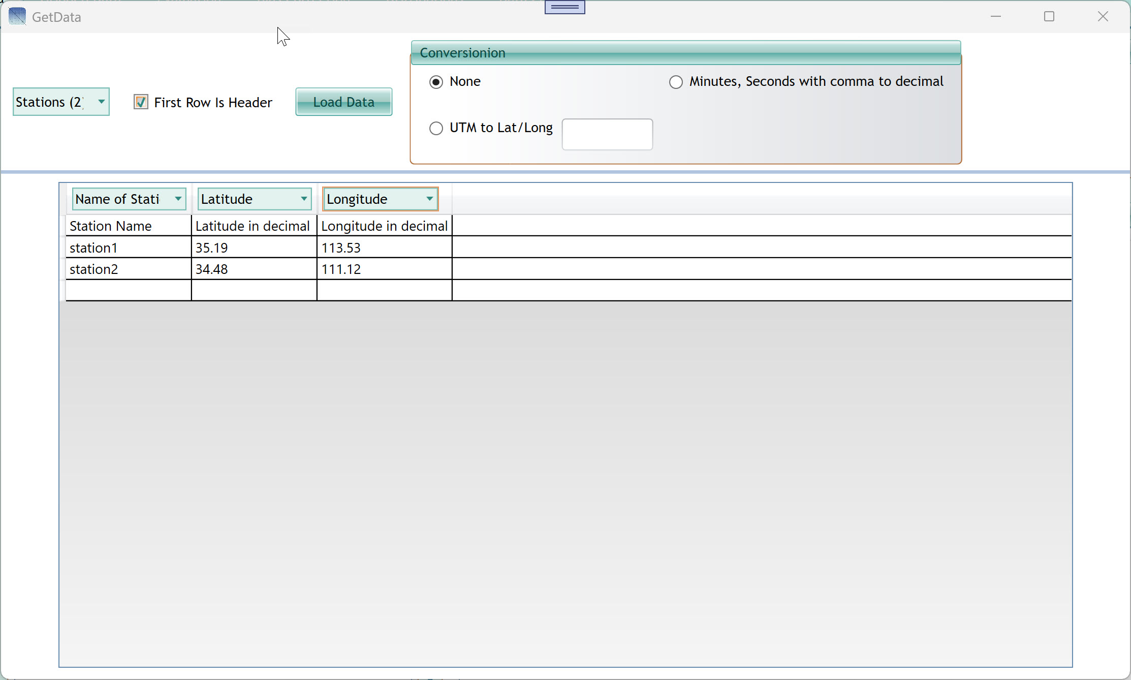
2.1 The GetData Window
The GetData window reads a text or CSV file that defines your
stations. Each row in the file represents one station with columns for
name, latitude, and longitude.
| Stations (N) dropdown |
Displays the number of stations detected from the file. After
loading, confirm this number matches your expectations. |
| First Row Is Header checkbox |
Check this if your file's first row contains column headings (e.g.
"Station Name", "Latitude", "Longitude"). Uncheck if the first row is
actual data. |
| Load Data button |
Read the file and populate the data grid below. Click this after
selecting your file and setting the options above. |
| Conversion — None |
Use coordinates exactly as they appear in the file (decimal degrees,
the standard format). |
| Conversion — Minutes, Seconds with comma to
decimal |
Automatically converts DMS (degrees-minutes-seconds with comma
separator) coordinates to decimal degrees. Use this if your coordinate
file uses the DMS format. |
| Conversion — UTM to Lat/Long + zone field |
Converts UTM (Universal Transverse Mercator) easting/northing pairs
to decimal degrees. Enter the UTM zone number in the accompanying text
field (e.g. 38 for UTM Zone 38N). |
| Column header dropdowns (Name of Station, Latitude,
Longitude) |
After loading, use these dropdowns to tell the tool which column in
your file corresponds to each field. The dropdown label appears above
each column in the data grid. If your file has a header row, the tool
may auto-map these. |
| Data grid (bottom half) |
Displays the file contents row by row after loading. Verify that
stations appear with the correct names and coordinates before closing.
In the example shown: station1 at 35.19°N, 113.53°E and station2 at
34.48°N, 111.12°E. |
Tip: Coordinates must be in decimal degrees (e.g. 35.19, not 35°11'24").
If your source data uses degrees-minutes-seconds, use the "Minutes,
Seconds with comma to decimal" conversion option.
Longitude values east of the prime meridian are positive; west are
negative. Latitude values north of the equator are positive; south are
negative.
The station names you enter here are used throughout the entire tool
— in evaluation charts, comparison tables, output files, and
distribution plots. Choose names that are short but
descriptive.
3. Station Data Tab
The Station Data tab is always the first tab you work with. Its
purpose is to load your observed historical weather data — the ground
truth that the bias-correction methods use as their calibration target.
This data typically spans 20–50 years of daily, monthly, or sub-daily
records from one or more ground-based weather stations.
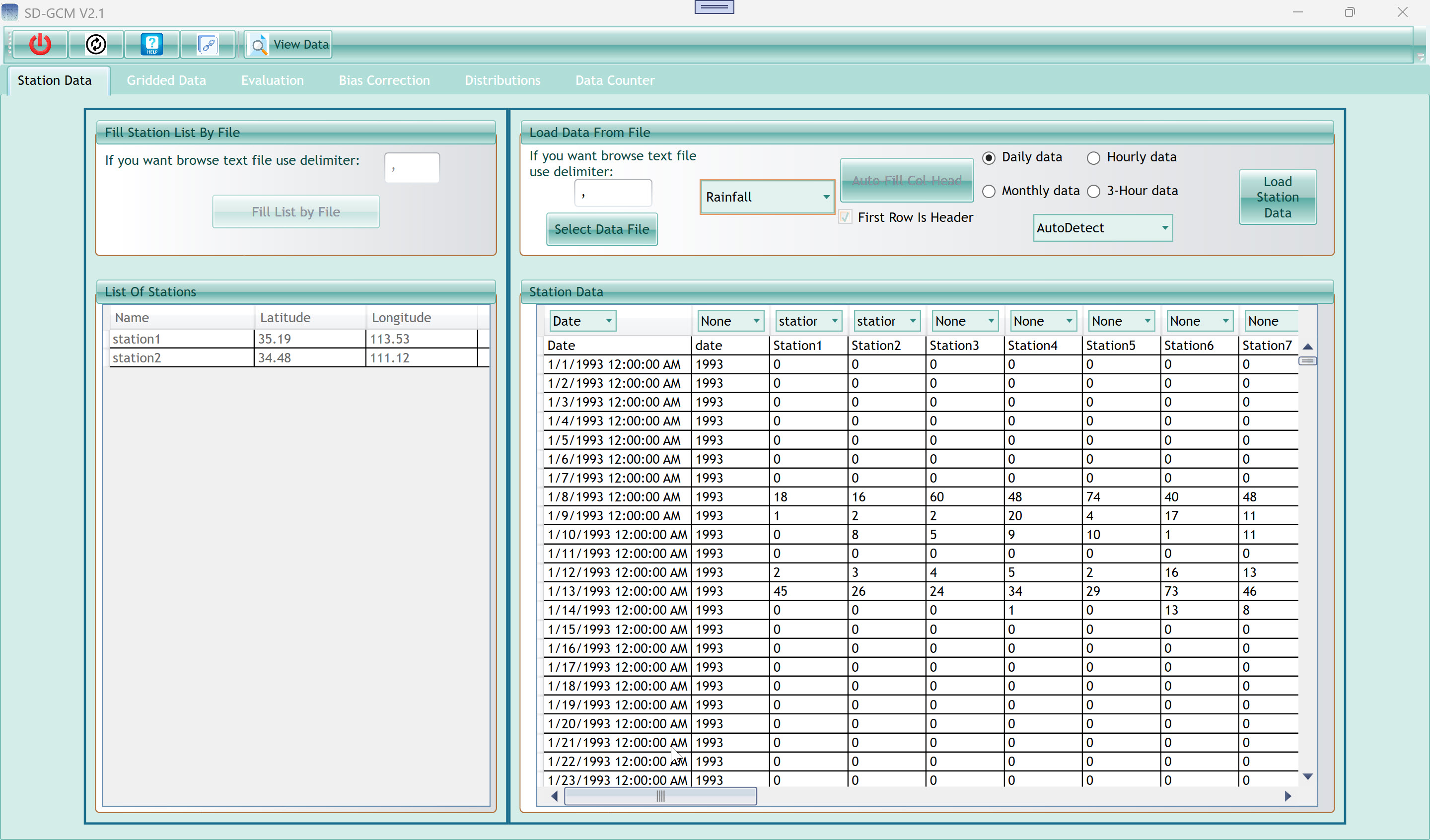
3.1 Left Panel — Fill
Station List By File
This panel lets you load the station list (names and coordinates)
from a delimited text file. Once the list is loaded here, it persists
for the entire session and drives the column assignment in the
data-loading panel on the right.
| Delimiter field (top) |
Type the character that separates columns in your station list file.
The default is a comma (,). Use a semicolon, tab (\t), or space as
needed. This delimiter applies only to the station list file, not to the
observation data file. |
| Fill List by File button |
Opens a file browser. Select your station list file (CSV or TXT).
The tool reads the file, parses it using the delimiter above, and opens
the GetData window (see Section 2) for coordinate assignment and
conversion. |
3.2 Left Panel — List Of
Stations
After loading, this table shows all stations currently registered.
Each row has three columns: Name, Latitude, and Longitude. You can
scroll down if you have more stations than are visible.
| Name column |
The station identifier as read from your file. This name is used in
all downstream analysis, charts, and export files. |
| Latitude column |
Decimal latitude of the station. Used to find the nearest GCM grid
cell when extracting data from NetCDF or CDS. |
| Longitude column |
Decimal longitude of the station. |
3.3 Right Panel — Load Data
From File
This is the main data-loading panel. It reads your observed
time-series data file and maps its columns to the station names in the
list.
| Delimiter field |
Column separator for the observation data file. Defaults to
comma. Change to match your file format before selecting the
file. |
| Select Data File button |
Opens a file browser to choose your observation data file. After
selecting, the file is read and displayed in the Station Data grid
below. Column assignment dropdowns appear above each column. |
| Sheet dropdown |
Select the Sheet name (climate variable) your data represents.
Options include Rainfall (precipitation), Temperature, and others. This
label is used in chart axis titles and output file names. It does not
affect calculation — the numerical values are used directly. |
| Daily / Hourly / Monthly / 3-Hour data radio
buttons |
Tell the tool what time step your station data has. This is
critical: it determines how the station data loads or how aggregates (or
not) for monthly calculations, how dates are interpreted, and how
evaluation periods are defined. Select exactly one according to your
station data in the Excel file. |
| Auto-Fill Col Head button |
After selecting a file, click this to automatically assign each
column to a station by matching the column header text to station names
in the list. If your file's column headers exactly match your station
names (case-insensitive), this saves manual assignment. Please recheck
it after filling |
| First Row Is Header checkbox |
Check if your data file has a header row. When checked, the first
row is used for the Auto-Fill feature but is not treated as a data
value. |
| Date format dropdown (AutoDetect) |
Select the date format used in your date column. AutoDetect tries
common formats automatically. If AutoDetect fails or produces wrong
dates, select your exact format: yyyy (year only, e.g. 1993),
MM/dd/yyyy, dd/MM/yyyy, yyyyMMdd, yyyyddd (Julian day), and others. See
the dropdown for the full list. When your file stores only the year
number (e.g. 1993 repeated 365 times), select yyyy explicitly. If you do
it wrong and no error happens, the year period combobox will be
wrong |
| Load Station Data button |
After assigning columns (Date and one or more station names) using
the dropdowns above each column, click this button to finalize loading.
The data is stored in memory and the tab becomes complete. |
3.4 The Station Data Grid
After selecting a file, a data grid appears in the lower-right area.
The top row of the grid shows column assignment dropdowns — one per
column. Use these to tell the tool what each column represents: Date, or
the name of a specific station. Set unused columns to None((if you have
selected before).
| Column dropdown (Date) |
Assign this to the column containing dates or year values. Exactly
one column must be assigned as Date. |
| Column dropdown (station name) |
Assign to columns containing station observation values. Each
station in your list should have one column assigned. Columns with no
matching station can be left as None. |
| Data rows |
Preview of your file contents. Verify that dates look correct and
that values are in the expected range. Missing values below -98 are
automatically treated as missing-value sentinels and excluded from
calculations. |
Note: The observation data must cover the calibration period you plan to
use in the Evaluation tab. A minimum of 10 years is recommended for
reliable transfer function estimation; 20+ years is ideal.
If you load multiple stations, all stations must share the same date
range and time step. Each station's column should be in the same unit as
specified by the Variable dropdown.
Missing values entered as -99 or any value below -98 are silently
skipped. The tool will ask whether to fill blank cells with the column
mean.
4. Gridded Data Tab
The Gridded Data tab is where you load the GCM output. You need two
separate GCM datasets: one covering the historical calibration period
(same era as your station observations) and one covering the future
projection period under an SSP or RCP scenario. The tab also contains
the Unit Converter, which handles the mismatch between GCM native units
and the units of your station data. If you load only historical data so,
you will have only the Evaluation tab activated.
Three radio buttons at the top let you choose how GCM data enters the
tool. Only one method is active at a time.
| Method 1 — Excel / CSV |
Load GCM data from Excel (.xlsx) or CSV files that you have already
prepared. Two buttons appear: Historical (Excel) and SSP/RCP (Excel),
one for each dataset. Use this if you already have extracted, formatted
GCM data as a spreadsheet. |
| Method 2 — CMIP6 OPeNDAP |
Download CMIP6 data directly from the Copernicus Climate Data Store
(CDS) over the internet. Click "Download CMIP6 (OPeNDAP)" to open the
Download CMIP6 window (see Section 5). This is the easiest method if you
have a CDS account and your stations are within a CMIP6 model's
domain. |
| Method 3 — NetCDF Files |
Load standard NetCDF (.nc) files directly. This is the most flexible
method and works with any CMIP6, CMIP5, or regional model output. Use
the "Select File" buttons in each section below to browse for your
files. This is the default selected method. |
4.2 Load Historical Data
This section loads the GCM historical simulation — the model's
representation of past climate, used to build the bias-correction
transfer function. It must overlap with your observation period.
4.2.1 Settings Sub-Panel
| Select File button |
Browse for and open a NetCDF file containing the historical GCM run.
After selecting, the filename appears in the adjacent dropdown, and the
View DB button activates. |
| File dropdown |
Shows the currently selected file. You can also type a path
directly. Editable in case you want to switch to a different file
without browsing. |
| View DB button |
Open a raw data viewer showing the contents of the selected file.
Use this to verify the file loaded correctly and to inspect variable
names, dimensions, and sample values. |
| Time (NetCDF var name field) |
The name of the time dimension variable in the NetCDF file. For most
CMIP6 files this is "time". If your file uses a different name (e.g. "t"
or "T"), enter it here if the tool cannot find it automatically. |
| Latitude field |
The name of the latitude dimension or variable. Usually "lat" or
"latitude" in CMIP6 standard files. Enter it here if the tool cannot
find it automatically. |
| Longitude field |
The name of the longitude dimension or variable. Usually "lon" or
"longitude". Enter it here if the tool cannot find it
automatically. |
| 4th Dim field (disabled) |
For 4-dimensional variables (e.g. pressure-level data with
dimensions time × level × lat × lon), enter the level dimension name.
The tool reads the first level index (index 0). This field is disabled
for standard surface variables. |
| Time Units field |
The time unit string from the NetCDF file's time variable
attributes. Format: "days", "hours", or "seconds". Copy this from the
file's metadata if the tool does not auto-populate it (e.g. from CDO
ncdump output). |
| Since field |
The reference date for the time axis, in YYYY-MM-DD format (e.g.
1850-01-01). This is the base date from which the time offset is
measured. |
| Calendar field |
The calendar system used by the GCM. Common values: standard
(Gregorian), 360_day (30-day months, used by many CMIP models), 365_day
or noleap (no leap years). The tool uses this to correctly reconstruct
calendar dates. |
4.2.2 Loading Sub-Panel
| GCM Model field |
A text label for the GCM model name (e.g. MPI-ESM1-2-HR). When
loading via CDS or if the filename follows CMIP6 conventions, this is
auto-populated. Otherwise type it manually. This label appears in
evaluation output and LLM export summaries. |
| Scenario field |
A text label for the experiment name (e.g. historical).
Auto-populated from CMIP6 filenames when possible. |
| Variable dropdown |
Select the CF variable name in the NetCDF file to extract (e.g. tas
for temperature, pr for precipitation). The dropdown is editable — type
directly if your variable is not listed. |
| Load Historical button |
Start the extraction process. The tool reads the NetCDF file, finds
the nearest grid cell to each station by lat/lon distance, and extracts
the time series for each station. Progress appears in the bar
below. |
| View button |
After loading, open a data viewer showing the extracted historical
GCM values for all stations. |
| Progress Bar checkbox |
Enable a visible progress bar during loading. Useful for large files
or many stations; disable for faster loading of small files. |
| Progress bar (0.0%) |
Shows extraction progress as a percentage (0–100%). Updates in real
time while loading. |
4.3 Load RCPs/SSPs Data
This section is identical in layout to Load Historical Data but loads
the future scenario simulation. All the same fields apply. The variable
name and calendar should match the historical file exactly. The time
range should cover your intended projection period (e.g. 2020–2100 for a
full SSP scenario).
4.4 Currently Loaded Status
Bar
At the bottom of the main panel, two read-only status lines confirm
what has been loaded:
| Historical: (none) / filename |
Shows the currently loaded historical GCM dataset name and period
once loading is complete. Displays "(none)" until data is loaded. |
| SSP/RCP: (none) / filename |
Shows the currently loaded future GCM dataset. Displays "(none)"
until loaded. |
4.5 Unit Converter (Right
Panel)
GCM NetCDF files store variables in SI units that often differ from
the units used in station observations. For example, temperature is
stored in Kelvin (K) in CMIP6 but your station data is in degrees
Celsius. Precipitation flux is stored in kg m⁻² s⁻¹ but your station
data is in mm/day. The Unit Converter applies a mathematical
transformation to every GCM value before it enters any bias-correction
calculation.
| No Conversion |
Use raw GCM values as-is. Select this when your GCM file is already
in the same units as your station data (e.g. if you pre-processed the
file externally). |
| Kelvin → °C |
Subtracts 273.15 from every GCM value. Use for temperature variables
(tas, tasmax, tasmin) when the GCM file is in Kelvin. |
| Flux → mm/day |
Multiplies every GCM value by 86400 (seconds per day). Use for
precipitation and evaporation variables stored as kg m⁻² s⁻¹ (equivalent
to mm/s), which is the CMIP6 standard for pr. |
| W/m² → hr/day |
Multiplies by 0.041674. Use for solar radiation (rsds) to convert
from W/m² to sunshine hours per day. |
| Multiply × (value) |
Applies a custom multiplication factor. Enter the factor in the text
field. Example: multiply by 0.01 to convert Pa to hPa, or by 1000 to
convert kg/kg to g/kg. |
| Plus + (value) |
Adds a constant offset. Enter the value in the text field. |
| Minus − (value) |
Subtracts a constant offset. |
| Correction Factor — Additive |
Tells the downscaling methods to treat this variable as additive
(appropriate for temperature, where biases are differences). The Delta
method will use subtraction; other methods will use the Normal
distribution. |
| Correction Factor — Multiplicative |
Tells the downscaling methods to treat this variable as
multiplicative (appropriate for precipitation, where biases are ratios
and negative values have no physical meaning). Negative corrected values
are clamped to zero. |
| Save Settings button |
Apply the selected unit conversion and correction factor to the
loaded GCM data. You must click this before running Evaluation or Bias
Correction. The conversion is applied once, internally, to both the
historical and future GCM datasets. |
| Tip text (bottom) |
A read-only reminder that wind speed (sfcWind) and relative humidity
(hurs) are already in standard units (m/s and %, respectively) and do
not need conversion. |
Tip: Always match units before running any analysis. The most common
errors in new analyses come from incorrectly set the unit converter. If
your evaluation metrics are wildly off (e.g. NSE = big negative), the
first thing to check is whether units are correctly set.
The correction factor choice (Additive vs Multiplicative) affects the
mathematical form of ALL six methods. Temperature is always Additive;
precipitation is always Multiplicative. Do not mix these up.
After clicking Save Settings, the status bar at the bottom of the
Gridded Data panel updates to confirm what is loaded. If it still shows
"(none)", the data was not loaded successfully before you tried to save
settings.
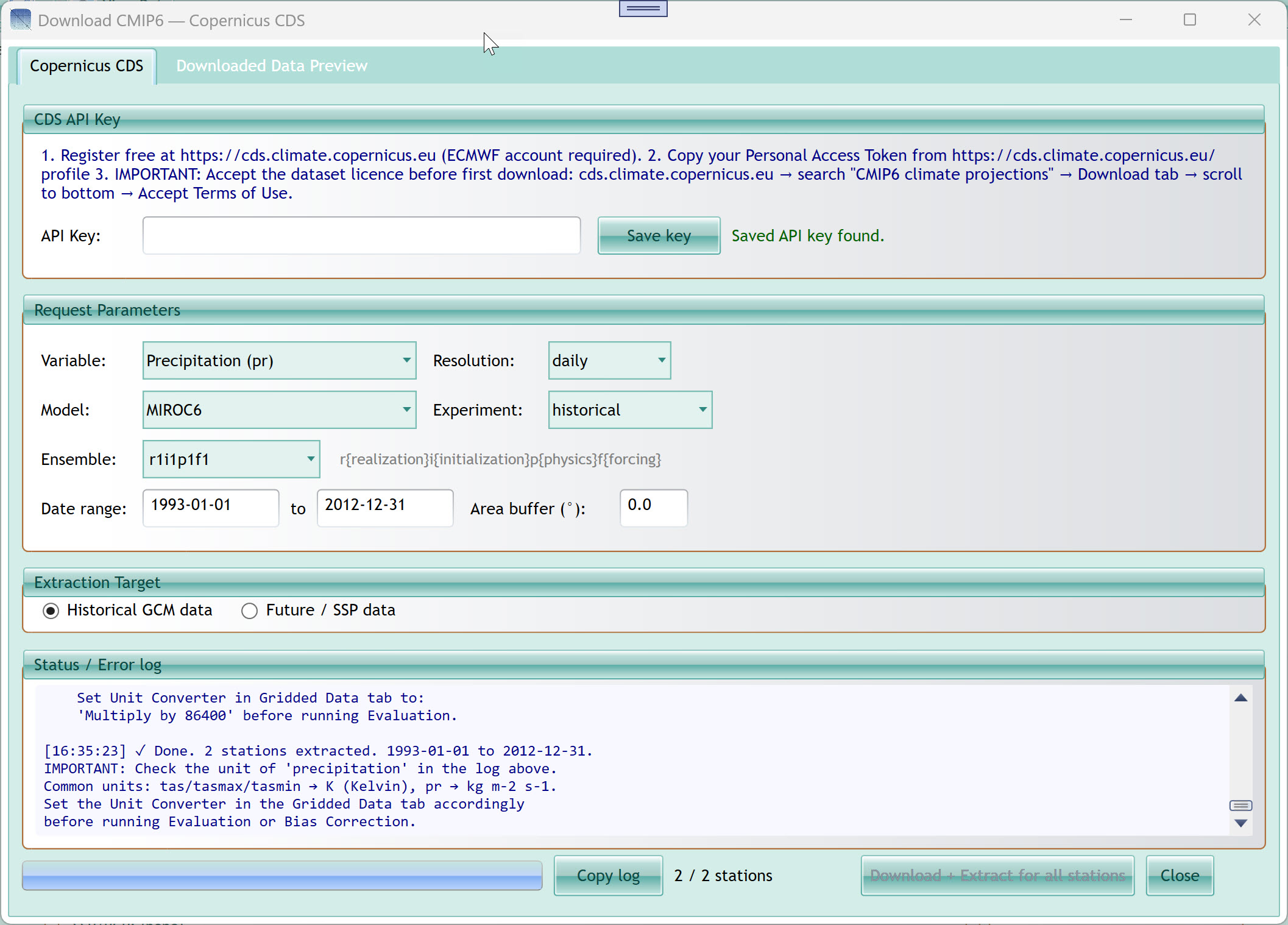
5. Download CMIP6 Window
(Copernicus CDS)
The Download CMIP6 window provides direct access to CMIP6 data from
the Copernicus Climate Data Store (CDS), operated by ECMWF on behalf of
the European Union. It eliminates the need to manually search, download,
and preprocess multi-gigabyte NetCDF files: the tool downloads only the
nearest grid cell time series for each of your stations. Open this
window by selecting Method 2 in the Gridded Data tab and clicking
"Download CMIP6 (OPeNDAP)".
5.1 Copernicus CDS Tab
5.1.1 CDS API Key Section
The CDS API uses a Personal Access Token for authentication. You need
a free ECMWF account to obtain one. The key is saved securely in the
Windows Credential Manager so you only need to enter it once.
| Instructions text |
Three-step setup guide shown in blue text: (1) Register at
cds.climate.copernicus.eu, (2) copy your Personal Access Token from the
profile page, (3) accept the dataset terms of use on the CDS website
before your first download. |
| API Key field (password box) |
Paste your CDS Personal Access Token here. The characters are hidden
for security. This is a plain UUID string (e.g.
d6fb36d7-e691-4a5f-974e-...), NOT the old UID:APIKEY format used before
2024. |
| Save key button |
Store the key in Windows Credential Manager. After saving, you will
not need to re-enter it in future sessions. The status label to the
right will confirm "Saved API key found." |
| Status label (Saved API key found.) |
Read-only confirmation of whether a key is stored. Green text means
a valid key is ready. Orange text with a warning means the stored key
may be in the old format and needs updating. |
Important: Before your first download, you must accept the CMIP6 dataset Terms
of Use on the CDS website. Log into cds.climate.copernicus.eu, search
for "CMIP6 climate projections", open the Download tab, scroll to the
bottom, and accept the licence. Downloads will fail with HTTP 403 if you
skip this step.
5.1.2 Request Parameters
Section
| Variable dropdown |
Select the climate variable to download. Categories include
Temperature (tas, tasmax, tasmin, ts), Precipitation & Hydrology
(pr, prsn, mrros, snw, evspsbl, mrso), Humidity (hurs, huss), Wind
(sfcWind, uas, vas), Radiation (rsds, rlds, rsus, rlus, rsdt, rsut,
rlut), and Sea Ice & Ocean (siconc, tos). The dropdown is grouped by
category for easier navigation. Separator items (greyed out) are
category labels, not selectable options. |
| Resolution dropdown |
Choose "daily" for daily time step data or "monthly" for monthly
means. Match this to your station data time step. Most bias-correction
workflows use daily data. |
| Model dropdown |
Select the GCM to download from. Available models include MIROC6,
CanESM5, MPI-ESM1-2-LR, MPI-ESM1-2-HR, IPSL-CM6A-LR, NorESM2-LM,
GFDL-ESM4, ACCESS-CM2, INM-CM5-0, CMCC-ESM2, BCC-CSM2-MR, CESM2,
EC-Earth3, and MRI-ESM2-0. Not all models have data for all variables
and experiments; the CDS will return an error if the combination does
not exist. |
| Experiment dropdown |
Select the CMIP6 experiment: "historical" (past climate, 1850–2014),
"SSP1-2.6" (low emissions), "SSP2-4.5" (intermediate), "SSP3-7.0"
(high), or "SSP5-8.5" (very high emissions, 2015–2100). |
| Ensemble dropdown |
Select the ensemble member (variant label). The default r1i1p1f1 is
the primary member for most models. The label format is
r{realization}i{initialization}p{physics}f{forcing}. If you need a
specific ensemble member for uncertainty analysis, select it here or
type a custom label directly (the field is editable). |
| Date range (start) |
Start date of the data request in YYYY-MM-DD format. For historical
data: 1850-01-01 to 2014-12-31. For SSP scenarios: 2015-01-01 to
2100-12-31. Enter dates that overlap with your station observation
period. |
| Date range (end) |
End date of the request, same format. Match this to your desired
calibration period end date (historical) or projection end date
(future). |
| Area buffer (°) field |
Extra degrees added around each station's lat/lon when defining the
bounding box sent to CDS. The tool internally enforces a minimum of 1.5°
to guarantee at least one GCM grid cell falls inside the box for any
model resolution. Enter 0 to use the minimum, or a larger value if you
want a wider spatial context. The tool always extracts only the nearest
grid point to the station regardless of buffer size. |
| Historical GCM data radio button |
After extraction completes, store the data as the Historical GCM
dataset. Select this when downloading a historical experiment run. |
| Future / SSP data radio button |
Store the extracted data as the Future SSP/RCP dataset. Select this
when downloading an SSP scenario run. |
5.1.4 Status / Error Log
The large text area at the bottom provides a real-time log of
everything the tool is doing. It shows timestamps, bounding box
coordinates, job submission URLs, job status polling updates, download
status, and any error messages. This is the primary diagnostic tool when
something goes wrong.
| Status log text area |
Read-only, scrollable log. Each entry is timestamped. Look here if a
download fails — the error message from CDS (e.g. HTTP 403 = terms not
accepted, HTTP 401 = wrong API key, HTTP 400 = invalid parameter
combination) is displayed here in full. The log also warns you when raw
GCM units differ from station units (e.g. pr is in kg m⁻² s⁻¹ and needs
×86400 conversion). |
| Copy log button |
Copy the entire log text to the clipboard with one click. Useful for
sharing error details when seeking support. On clipboard conflicts, a
fallback dialog opens showing the text for manual selection. |
| N / N stations label |
Shows progress as station downloads complete (e.g. "2 / 2
stations"). Updates after each station finishes. |
| Progress bar |
Visual progress bar filling from left to right as stations are
processed. |
| Download + Extract for all stations button |
Start the download process for all stations in your list. Each
station is processed sequentially: a CDS job is submitted, the tool
polls for completion, downloads the resulting zip, extracts the NetCDF,
reads the nearest grid cell values, and moves to the next station. This
can take several minutes per station depending on CDS queue depth. |
| Close button |
Close the Download CMIP6 window and return to the main application.
The downloaded data remains loaded in memory. |
5.2 Downloaded Data Preview
Tab
After a successful download, switch to the Downloaded Data Preview
tab to verify the extracted values before using them in analysis.
| Station dropdown |
Select which station's downloaded data to preview. |
| Info label |
Shows the number of values and the date range of the extracted
series (e.g. "7305 values (1993-01-01 to 2012-12-31)"). |
| Data grid |
Two columns: Date (YYYY-MM-DD format) and Value (raw GCM value in
the file's original units, without unit conversion applied — conversion
is set separately in the Gridded Data tab). Scroll through to spot any
unexpected NaN values or unrealistic numbers. |
Tip: CDS jobs are queued on ECMWF servers and may take from 30 seconds to
30 minutes depending on server load. The tool polls every 5–10 seconds
and waits up to 120 minutes. If a download times out, check the CDS
website (cds.climate.copernicus.eu/requests) to see the job status.
Raw CDS data for precipitation is in kg m⁻² s⁻¹. After downloading,
remember to set the Unit Converter in the Gridded Data tab to "Flux →
mm/day" (multiply by 86400) before running Evaluation. The status log
will display a unit warning to remind you.
If you need both historical and SSP data, run the tool twice: once
with "Historical GCM data" selected and once with "Future / SSP data"
selected, changing the Experiment and Date range each time.
6. Evaluation Tab
The Evaluation tab is where you determine which bias-correction
method performs best for your specific combination of GCM and station
data. The key principle is cross-validation: you withhold part of the
historical record (the evaluation period) from calibration, apply each
method trained only on the calibration period, and compare the corrected
output to the actual observations during the withheld period. This gives
an honest estimate of how the method will perform when applied to the
future.
6.1 Evaluation Downscaling
GroupBox
6.1.1 Calibration &
Evaluation Periods
These six dropdowns define three non-overlapping (or overlapping, but
logically distinct) time periods drawn from the historical GCM data.
| Observation Period (start, end) |
The years of your station observation data to use. All station
values outside this range are ignored. Set this to match the full span
of your reliable station record. |
| Historical GCM Period (start, end) |
The years of historical GCM data to use for building the transfer
function (calibration). This should overlap with the Observation Period.
Common practice: use the full overlap period (e.g. 1993–2002 in the
screenshot). |
| Evaluation Period (start, end) |
A separate period, also drawn from the historical GCM record, used
to test the method. The bias-correction is applied to the GCM data in
this period and compared to the corresponding observed values.
Crucially, this period should NOT overlap with the Historical GCM Period
to ensure a genuine out-of-sample test. Example: calibrate on 1993–2002,
evaluate on 2003–2012. |
Tip: Split your historical record approximately 60/40 or 70/30 between
calibration and evaluation. With 20 years of data, a common split is 12
years calibration + 8 years evaluation.
The Evaluation Period can overlap with the calibration period if you
want to check in-sample fit (how well the method matches its own
training data). However, for a meaningful comparison of methods, always
use a separate, non-overlapping evaluation period.
All period dropdowns are populated automatically from the date range
of your loaded data. If a year you need does not appear, check that your
data was loaded correctly and covers that year.
Six radio buttons let you select which method to evaluate. Only one
method runs per click of the Evaluate button.
| Delta |
The simplest method. Corrects the GCM mean by a multiplicative ratio
(precipitation) or additive shift (temperature) computed from the
calibration period. Fast and interpretable, but only corrects the mean —
it does nothing about variability, skewness, or distributional
shape. |
| QM (Quantile Mapping) |
Maps each GCM value to the corresponding observed quantile using
parametric distributions (Normal for temperature, empirical for
precipitation). Corrects both mean and distributional shape
simultaneously. |
| EQM (Empirical Quantile Mapping) |
Fully non-parametric variant of QM. For temperature, uses empirical
CDFs from the sorted data instead of fitting a Normal distribution. For
precipitation, identical to QM in V2.1. More flexible than QM for
non-Normal temperature distributions. |
| QDM (Quantile Delta Mapping) |
Preserves the GCM's projected change signal at every quantile, not
just the mean. Computes a quantile-specific delta (how much each
quantile changes between historical and future) and adds it to the
observed value at that quantile. Recommended for future projections
where distributional changes matter. |
| DQM (Detrended Quantile Mapping) |
Removes the mean trend from the future GCM before applying EQM, then
reapplies the trend. Simpler than QDM but only preserves the mean change
signal. A good balance between correction quality and complexity. |
| SDM (Scaled Distribution Mapping) |
Specifically designed for precipitation. Corrects wet-day frequency
by ranking future GCM wet days and mapping them to observed wet days.
Explicitly resolves the "drizzle bias" — GCMs producing too many
light-rain days. Recommended for precipitation bias correction. |
6.1.3 Monthly Stratification
Checkbox
Monthly Stratification is a wrapper that applies the
selected method independently to each of the 12 calendar months. When
checked, the method is run 12 separate times: once for January data,
once for February data, etc. The resulting method name gets an _M suffix
(e.g. Delta_M, QDM_M, SDM_M).
Use Monthly Stratification when the GCM bias varies by season — for
example, a model that overestimates summer precipitation but
underestimates winter precipitation. Without stratification, a single
transfer function would partially correct one season while worsening the
other.
Tip: For most precipitation datasets, SDM_M or QDM_M with Monthly
Stratification gives the best results on independent evaluation
periods.
Monthly Stratification requires at least ~5 years in the calibration
period to estimate a reliable transfer function for each month. With
fewer years, the method may overfit to the calibration period.
| Evaluate button |
Run the selected method (with or without Monthly Stratification) on
the defined periods. The corrected time series is computed and displayed
in the chart below. Progress appears in the bar beneath the button. |
| Add to Comparison button |
Add the results of the current evaluation run to the Method
Comparison table at the bottom of the tab. Click this after each method
to build up a comparison. The button is disabled until at least one
Evaluate run has completed. After adding, the status text to the right
confirms the entry (e.g. "SDM_M added to comparison table."). |
| Progress bar (100%) |
Fills during evaluation computation. Returns to 100% when complete.
The calculation is fast (typically under 5 seconds for daily data) even
with Monthly Stratification. |
| Status text (red) |
Displays confirmation messages when a result is added to the
comparison table. Read-only. |
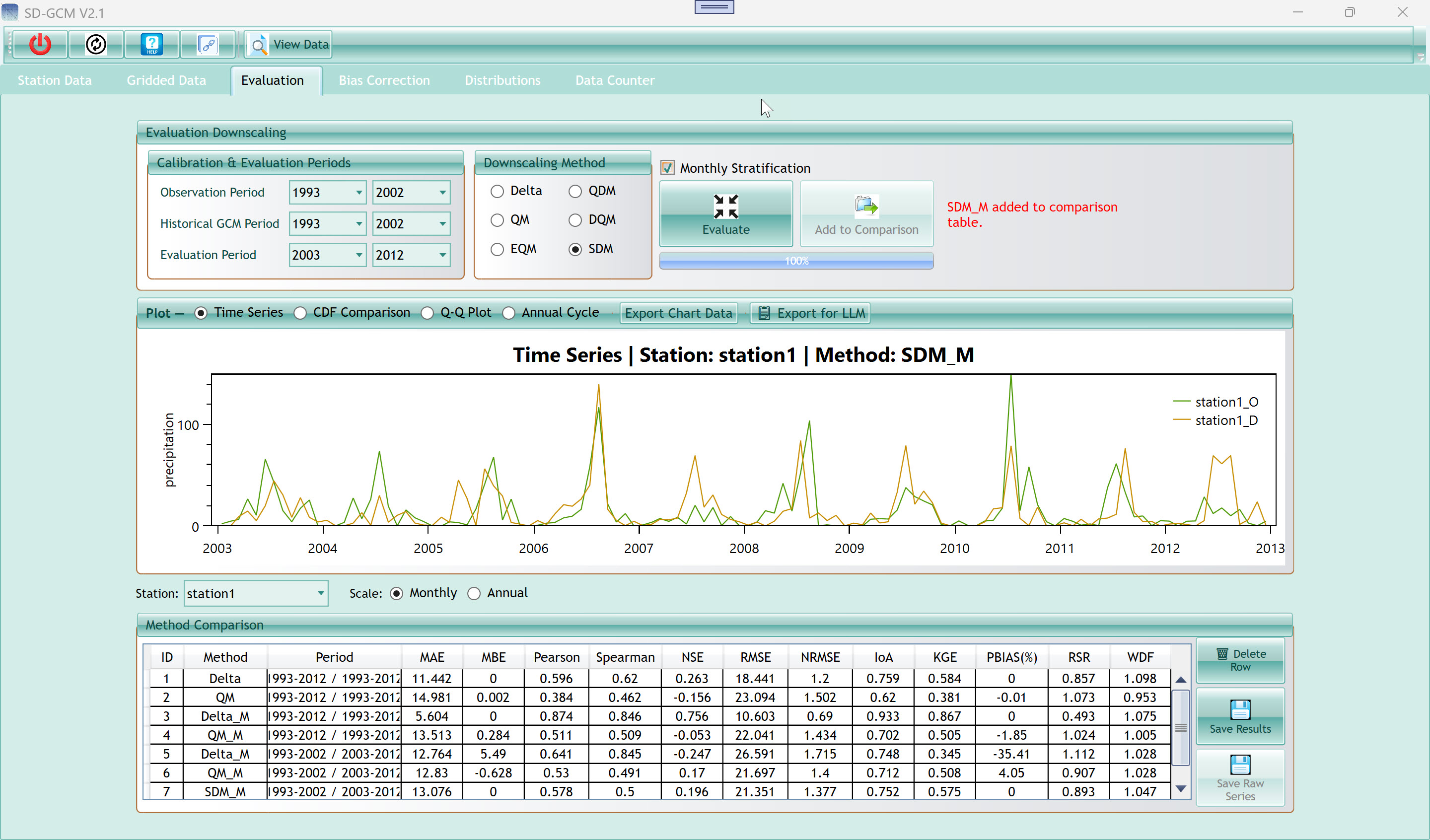
6.2 Plot Panel
The chart below the method selector shows a visual comparison of the
corrected output (orange, labelled _D for "downscaled") against the
observed station data (green, labelled _O for "observed") over the
evaluation period.
| Plot type — Time Series |
Shows monthly or annual aggregated values as a line chart over the
evaluation period. Gives an overall visual impression of how well the
corrected series tracks the observations. |
| Plot type — CDF Comparison |
Shows the empirical cumulative distribution functions of the
corrected and observed series on the same axes. A perfect correction
produces overlapping CDFs. Deviations indicate remaining bias at
specific quantiles. |
| Plot type — Q-Q Plot |
Quantile-quantile plot: each point is a paired quantile from the
corrected vs observed distributions. Points on the 1:1 diagonal line
indicate perfect quantile-level agreement. Curves above or below the
diagonal reveal over- or under-correction at those quantiles. |
| Plot type — Annual Cycle |
Bar chart showing mean values by calendar month for both corrected
(orange) and observed (green) series. Use this to diagnose seasonal bias
patterns — if the bars differ only in specific months, Monthly
Stratification may help. |
| Export Chart Data button |
Export the data behind the currently displayed chart to an Excel
file. Useful for creating custom figures in external tools. |
| Export for LLM button |
Generate a structured Markdown text file containing per-station
statistics, evaluation metrics, and a pre-written prompt asking an AI
assistant to interpret the results and write a Methods paragraph. Open
the resulting file in any text editor or AI chat window. |
| Station dropdown |
Select which station's data to display in the chart. Switch between
stations to compare their individual correction quality. |
| Scale — Monthly / Annual radio buttons |
Aggregate the time series to monthly means (more detail) or annual
means (cleaner long-term trends) before plotting. Does not affect the
calculated metrics. |
6.3 Method Comparison Table
Each time you click "Add to Comparison", a new row is appended to
this table showing the performance of that method run.
| MAE |
Mean Absolute Error — average magnitude of errors. Lower is
better. |
0 |
| MBE |
Mean Bias Error — average signed error. Positive = overestimation.
Zero is perfect. |
0 |
| Pearson |
Pearson correlation coefficient — linear temporal agreement. |
1 |
| Spearman |
Rank-based correlation — agreement in the ordering of values. |
1 |
| NSE |
Nash-Sutcliffe Efficiency — how much better the model is than the
observed mean as a predictor. NSE > 0.5 is generally acceptable; >
0.75 is good. |
1 |
| RMSE |
Root Mean Square Error — penalises large errors more heavily than
MAE. |
0 |
| NRMSE |
RMSE normalised by the observed mean. Allows comparison across
stations with different mean values. |
0 |
| IoA |
Index of Agreement (Willmott's d) — ranges 0–1; less sensitive to
outliers than NSE. |
1 |
| KGE |
Kling-Gupta Efficiency — decomposes into correlation, variability
bias, and mean bias. Values above −0.41 are better than the observed
mean benchmark. |
1 |
| PBIAS(%) |
Percent Bias — percentage overestimation (+) or underestimation (−)
of total volume. |
0% |
| RSR |
RMSE / standard deviation of observations. RSR < 0.7 is
considered acceptable. |
0 |
| WDF |
Wet-Day Frequency Ratio (precipitation only) — ratio of corrected to
observed wet-day counts. 1 = perfect frequency. |
1 |
| ID column |
Sequential row number, assigned in the order results were
added. |
| Method column |
Name of the method and stratification mode (e.g. SDM_M). |
| Period column |
Shows the calibration period and evaluation period used for this row
(e.g. 1993-2012 / 2003-2012). |
| Delete Row button |
Remove the selected row from the comparison table. Select a row by
clicking it, then click Delete Row. |
| Save Results button |
Export the complete comparison table to an Excel file with all
metrics for all stations and all methods. |
| Save Raw Series button |
Export the raw time series data (observed, historical GCM, and
corrected) to an Excel file at the original daily or monthly time step.
Useful for further analysis in R, Python, or other tools. |
Tip: Run all six methods with and without Monthly Stratification before
deciding. It only takes a few minutes. A common finding sample is that
SDM_M or QDM_M performs best for precipitation on independent periods,
while Delta_M performs surprisingly well for temperature.
KGE is often more informative than NSE because it separately
quantifies correlation, variability bias, and mean bias. A method with
high NSE but poor KGE may match the mean well but underestimate
variability.
WDF (Wet-Day Frequency Ratio) is only meaningful for precipitation. A
WDF > 1 means the corrected series has more rainy days than observed
— a common GCM drizzle bias that SDM is specifically designed to
correct.
7. Bias Correction Tab
The Bias Correction tab applies the method you selected in the
Evaluation tab to the full future SSP/RCP GCM dataset, producing your
final downscaled output. Unlike the Evaluation tab (which tests on
historical data), the Bias Correction tab trains on the complete
historical calibration period and projects onto the future period.
7.1 Left Panel — Evaluation
Downscaling
7.1.1 Downscaling Period
| Station Period (start, end) |
Years of your station observation data used for training the
transfer function. Set this to the full reliable observation
record. |
| Historical Period (start, end) |
Years of historical GCM data used for calibration. Should match or
overlap the Station Period. |
| Downscale Period (start, end) |
The future period to correct. These years are drawn from the loaded
SSP/RCP dataset. Set to whatever future period you want in your final
output (e.g. 2020–2035 or 2015–2100). |
7.1.2 Downscaling Method
The same six method radio buttons as in the Evaluation tab. Select
the method you determined was best in the Evaluation step.
7.1.3 Monthly Stratification
Checkbox
Same as in Evaluation. When checked, the method runs separately for
each calendar month. The output is labelled with the _M suffix in chart
titles and saved file names.
| Downscale button |
Run the bias correction. The tool trains the transfer function on
the station + historical GCM data covering the Station Period and
Historical Period, then applies it to all future GCM values in the
Downscale Period. A progress bar fills during computation. |
| Save DownScaled Data button |
Save the full bias-corrected future time series to an Excel file.
Columns: Date, Station1, Station2, ... with one row per time step. This
is the primary output file for downstream impact modelling. |
| Save Hourly or 3Hour Data button |
Available if your input data was hourly or 3-hourly. Saves the
output at the original sub-daily time step (the main save button
aggregates to daily). |
| Progress bar (100.0%) |
Shows computation progress. Fills quickly; reaches 100% when
done. |
7.2 Right Panel — Chart and
Controls
7.2.1 Station and Scale
Selectors
| Station dropdown |
Select which station to display in the chart. |
| Scale — Raw / Monthly / Annual radio buttons |
Choose the aggregation level for the chart: Raw (every time step),
Monthly (monthly means), or Annual (annual means). Affects only the
chart display, not the saved data. |
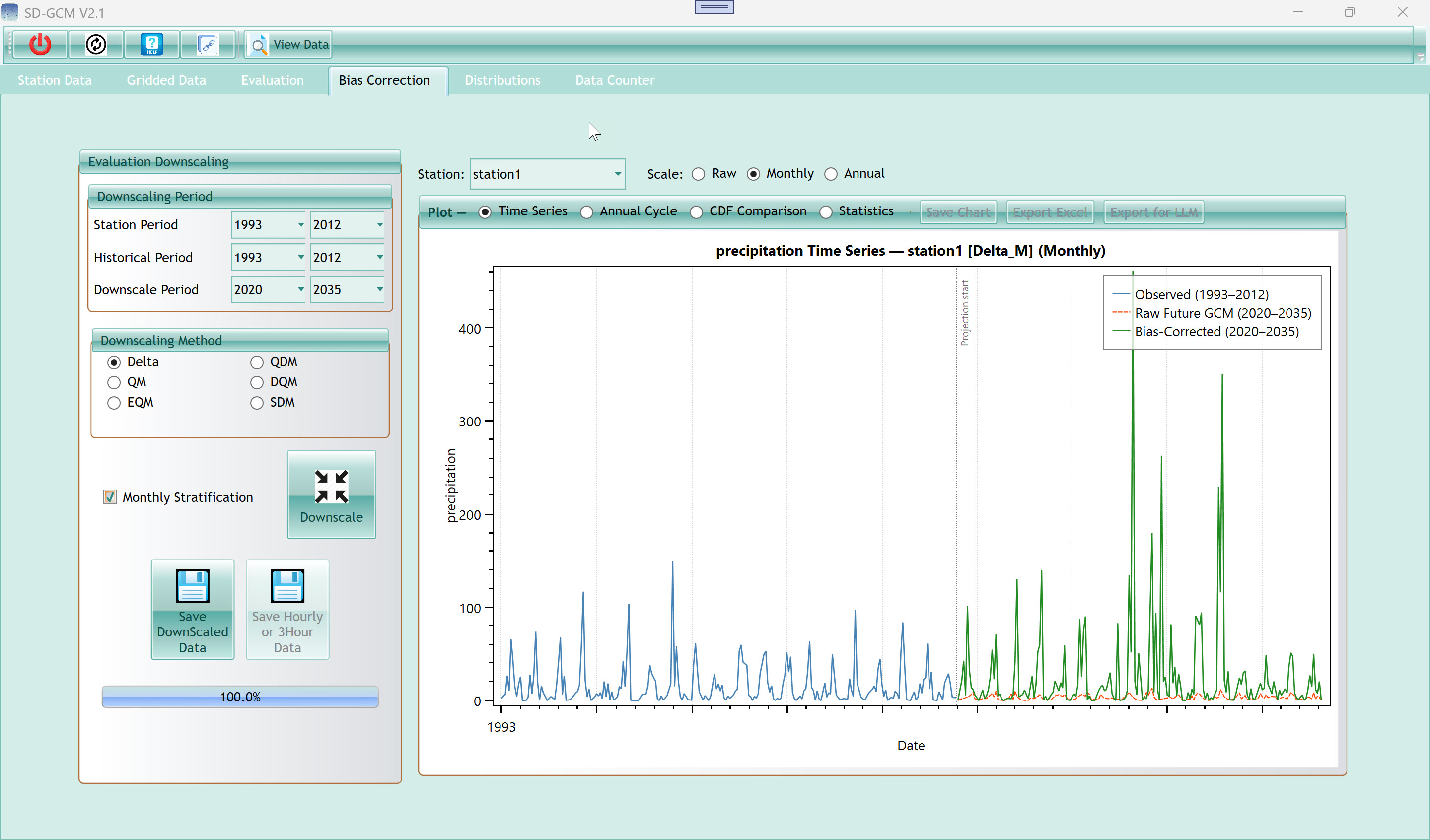
| Time Series |
Line chart showing three series: Observed (blue, calibration
period), Raw Future GCM (red dashed, projection period), and
Bias-Corrected (green, projection period). A vertical dotted line marks
the start of the projection period. This is the most informative view
for a quick visual check of the correction quality and the GCM change
signal. |
| Annual Cycle |
Grouped bar chart showing mean monthly values (Jan–Dec) for each of
the three series. Use this to check whether seasonal patterns in the
corrected data match the observed climatology. |
| CDF Comparison |
Empirical CDFs of all three series overlaid. Check that the
corrected (green) CDF closely follows the observed (blue) CDF shape,
especially in the tails. |
| Statistics |
Bar chart showing summary statistics (mean, standard deviation, CV,
min, max, P10, P50, P90) for each series. Confirms that the
bias-corrected output has statistics similar to the observations. |
| Save Chart button |
Save the currently displayed chart as a PNG or SVG image file. |
| Export Excel button |
Export the data series shown in the current chart to an Excel
file. |
| Export for LLM button |
Generate a structured analysis summary for AI-assisted
interpretation, similar to the button in the Evaluation tab. |
Tip: Always inspect the Time Series chart after running bias correction.
The most important visual check is that the green (corrected) line does
not simply mirror the blue (observed) line into the future — it should
show the GCM's projected change while having the distributional shape of
the observations.
If the Raw Future GCM (red dashed) is nearly flat at zero for
precipitation, the GCM raw values are in SI units (kg m⁻² s⁻¹) and need
the Flux → mm/day unit conversion. Return to the Gridded Data tab and
set the converter.
The projection start marker (vertical dotted line in the Time Series
chart) appears at the boundary between the calibration and projection
periods. Values to the left of it are the observed station data; values
to the right are the model output.
8. Distributions Tab
The Distributions tab provides two tools for probability distribution
analysis. The upper section ("Find Distributions") opens the
Distribution Fitting window to rank candidate distributions against your
data using formal goodness-of-fit tests. The lower section ("CDF/PDF
Plot") draws empirical and fitted CDF or PDF curves directly in the main
window for visual comparison across stations and periods.
8.1 Find Distributions Section
| Station dropdown |
Select which station's data to analyse. |
| Use Monthly Data checkbox |
When checked, the data is aggregated to monthly totals/means before
fitting. Strongly recommended for daily precipitation because fitting a
distribution to thousands of daily values (including many zeros) rarely
produces a useful result — monthly aggregates are more tractable and
more relevant for most applications. |
| Use Raw Data radio button |
Use the raw (all-year) time series from the selected source. |
| Use Maximum of Years radio button |
Take only the annual maximum value from each year, creating a series
of annual maxima. Use this for extreme value analysis (flood frequency,
drought analysis) where you want to fit a Gumbel or GEV distribution to
the series of annual peaks. |
| Use Minimum of Years radio button |
Take only the annual minimum value per year. Use for drought or
low-flow analysis. |
| Use Downscaled Data radio button |
Analyse the bias-corrected output from the Bias Correction tab. |
| Use Observation Data radio button |
Analyse the observed station data. Useful for understanding the
natural distribution of your variable before correction. |
| Check 12 Distributions button |
Open the Distribution Fitting window (see Section 8.2 below) and
automatically fit all available distributions to the selected data,
ranking them by the Anderson-Darling goodness-of-fit statistic. |
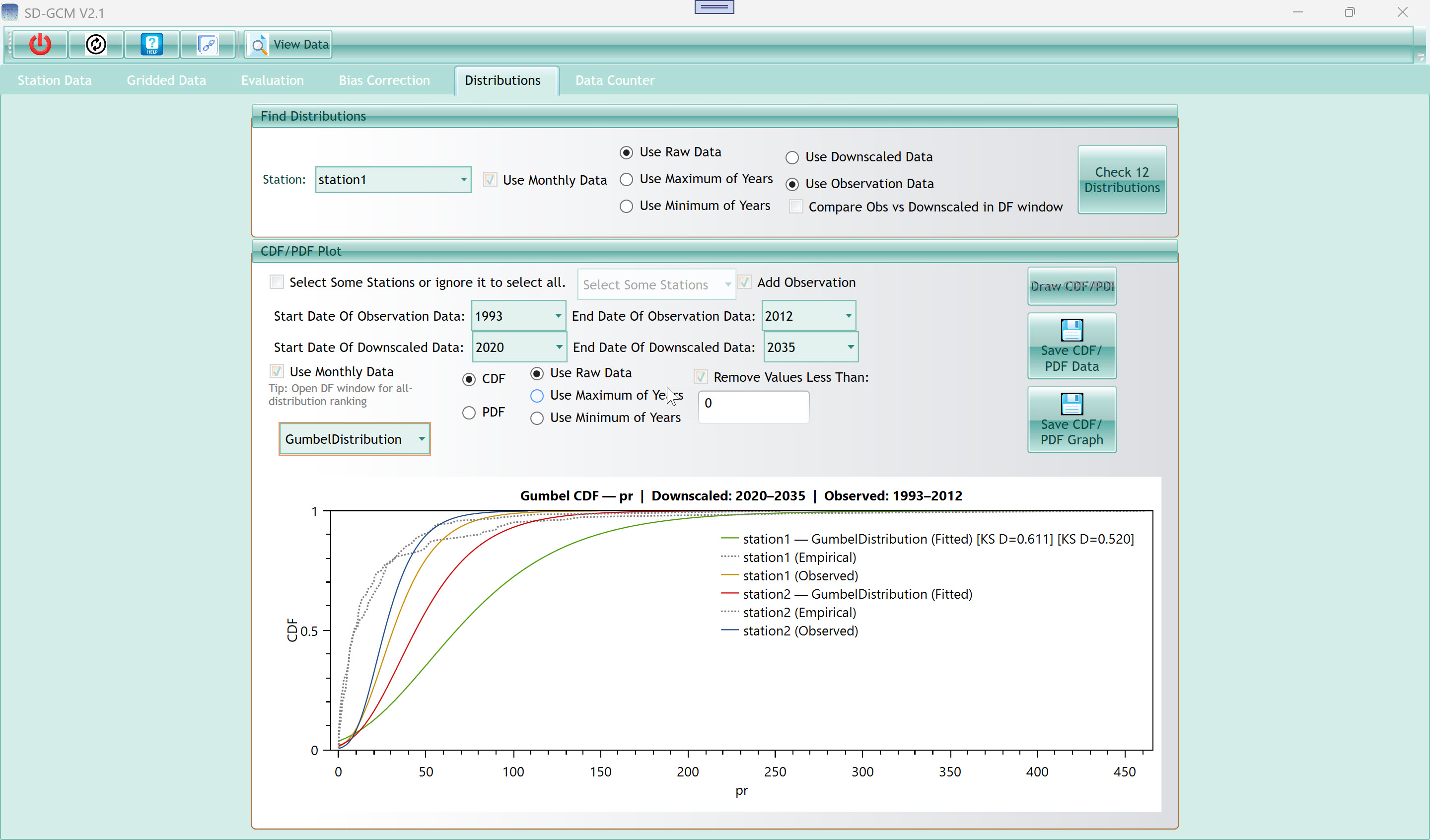
8.2 CDF/PDF Plot Section
| Select Some Stations checkbox + dropdown |
When the checkbox is unchecked (default), all stations are included
in the plot. Check the box and use the dropdown to select a specific
subset of stations to compare. |
| Add Observation checkbox |
Overlay the observed station data CDF/PDF on the same chart
alongside the downscaled data. Essential for checking whether the bias
correction has successfully matched the observed distribution. |
| Start/End Date Of Observation Data dropdowns |
Filter the observation period shown in the chart. Defaults to the
full loaded observation range. |
| Start/End Date Of Downscaled Data dropdowns |
Filter the downscaled projection period shown in the chart. |
| Use Monthly Data checkbox |
Aggregate data to monthly values before plotting. Recommended for
daily precipitation. |
| CDF radio button |
Plot the cumulative distribution function: y-axis = probability
(0–1), x-axis = variable value. Shows the full distribution shape and is
easier to read than PDF for skewed data. |
| PDF radio button |
Plot the probability density function: y-axis = density, x-axis =
variable value. Easier to see the mode and shape but harder to read
tails. |
| Use Raw Data / Maximum of Years / Minimum of Years radio
buttons |
Same as in the Find Distributions section — select the data
aggregation mode. |
| Remove Values Less Than checkbox + value field |
Filter out values below a threshold before fitting and plotting.
Useful for precipitation where you want to exclude dry days (e.g. set to
0.1 mm/day to work only with wet days). The default value is 0. |
| Distribution dropdown |
Select which theoretical distribution to fit and overlay. Options
include Exponential, Gamma, Gumbel, HyperbolicSecant, InverseGamma,
Logistic, LogLogistic, Lognormal, Normal, and Pareto. The empirical CDF
of the data is always shown (dotted line) regardless of which
distribution is selected. |
| Draw CDF/PDF button |
Compute the selected distribution fit and render the chart. The
chart title confirms the distribution name, variable, and date ranges.
Each station gets its own fitted line (solid, coloured), empirical CDF
(grey dotted), and — if Add Observation is checked — observed series
(gold). The KS D-statistic is shown in the legend next to the fitted
line name. |
| Save CDF/PDF Data button |
Export the chart data (empirical CDF points and fitted curve values)
to an Excel file. |
| Save CDF/PDF Graph button |
Save the chart as an image file (PNG or SVG). |
| Tip text (small, grey) |
Reminder: "Open DF window for all-distribution ranking" — referring
to the Check 12 Distributions button above. |
Tip: For precipitation, the Gamma distribution is the classical choice for
monthly totals. For annual maxima of precipitation or streamflow, the
Gumbel (Extreme Value Type I) distribution is widely used in engineering
frequency analysis.
The KS D-statistic shown in the legend is the maximum absolute
difference between the empirical and fitted CDFs. Smaller is better. A
D-value below 0.1 generally indicates a good fit; above 0.2 suggests the
distribution does not match the data well.
For temperature, the Normal distribution is usually the best choice
for monthly means. For daily temperature, a slightly skewed distribution
such as Logistic or GeneralizedNormal may fit better in extreme
climates.
9. Distribution Fitting Window
The Distribution Fitting window opens when you click "Check 12
Distributions" in the Distributions tab. It automatically fits a
comprehensive set of continuous probability distributions to your data
and ranks them by the Anderson-Darling goodness-of-fit statistic — the
most appropriate criterion for hydro-climate data because it gives
greater weight to distribution tails, where extreme events occur. The
window has two tabs.
9.1 Goodness-of-Fit Rankings
Tab
9.1.1 The Info Bar
The orange/amber banner at the top explains the ranking criterion:
"Ranked by Anderson-Darling statistic (lower = better fit).
Anderson-Darling is preferred for hydro-climate data: it weights
distribution tails more heavily than KS, making it sensitive to extremes
(floods, droughts). Chi-Square depends on arbitrary binning and is least
reliable for continuous data." This is read-only scientific context.
9.1.2 The Rankings Table
| Rank column |
Integer rank from 1 (best fit) to the number of successfully fitted
distributions. Distributions that failed to converge or produced invalid
statistics are ranked 999. |
| Distribution column |
Name of the fitted distribution. |
| AD Statistic (rank basis) column |
The Anderson-Darling test statistic value (A²). Lower values
indicate better agreement between the fitted distribution and the data,
especially in the tails. This is the primary ranking criterion. |
| Anderson-Darling Test column |
Detailed test output: Statistic value, Significant (True/False
indicating whether the distribution is rejected at 5% level), P-Value,
and Sign-Level. "Significant:False" means the distribution cannot be
rejected at the chosen significance level — this is a good sign.
"PValue:NaN" typically indicates a distribution that could not be tested
formally (see Notes column). |
| KS Statistic column |
The Kolmogorov-Smirnov D-statistic — the maximum absolute difference
between the empirical and fitted CDFs at any point. Useful as a
secondary check but less sensitive to tails than Anderson-Darling. |
| KS Test Detail column |
Detailed KS test output: Statistic, Significant, P-Value,
Sign-Level. Interpretation same as for the AD test column. |
| Chi-Square Test column |
Chi-Square test output. This test requires discretising the
continuous data into bins, making it less reliable than AD or KS. Use as
a supporting reference only. |
| Fitted Parameters column |
The estimated distribution parameters after fitting. For example, a
Gamma distribution shows k (shape) and θ (scale); a Normal shows μ
(mean) and σ² (variance). These parameters fully define the fitted
distribution for further use. |
| Notes column (red) |
Displays "This distribution has an error." in red for distributions
that failed to fit or produced invalid outputs (shown as rank 999). This
is normal for some distributions that are inappropriate for the current
data (e.g. Lognormal fails if data contains zeros or negatives). |
Click any row to automatically switch to the Best Fit Chart tab and
display that distribution's chart, making it quick to visually inspect
any distribution in the table.
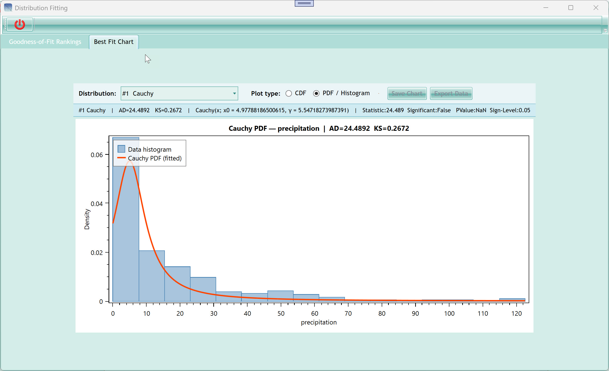
9.2 Best Fit Chart Tab
This tab shows a visual representation of a single chosen
distribution fitted to the data, either as a CDF comparison or a PDF +
histogram overlay.
| Distribution dropdown |
Select which distribution to visualise. The dropdown is pre-filled
with all successfully ranked distributions, listed in rank order (best
first, e.g. "#1 Cauchy", "#2 NakagamiDistribution"). Clicking a row in
the Rankings tab auto-selects the matching entry here. |
| Plot type — CDF radio button |
Show the fitted CDF (orange solid line) overlaid on the empirical
CDF (grey dotted line). Perfect alignment means the distribution fits
the data across the full range. The x-axis represents the variable
value; y-axis is cumulative probability (0–1). The x-axis is clipped at
the 1st and 99th percentile of the data to prevent outliers from
stretching the axis. |
| Plot type — PDF / Histogram radio button |
Show the fitted probability density function (orange solid curve)
overlaid on a histogram of the data (blue bars, density-normalised). The
histogram uses √n bins (where n is the sample size, capped between 10
and 50 bins) for a natural bin count. |
| Save Chart button |
Save the current chart as a PDF or SVG file to your chosen
location. |
| Export Data button |
Export the chart data to a 3-sheet Excel file: (1) Empirical CDF
points with variable values and cumulative probabilities, (2) fitted
curve values (300 evenly-spaced x-values with fitted CDF or PDF values),
(3) Summary sheet with distribution name, fitted parameters, AD and KS
statistics, and data range. Useful for reporting or creating
publication-quality figures. |
| Info panel (green bar) |
Displays a summary for the selected distribution: rank, AD
statistic, KS statistic, fitted parameters, and Anderson-Darling test
detail. All on one read-only line. |
| Chart area |
The OxyPlot chart. Hover to see data point coordinates. Resize the
window to expand the chart. The chart title follows the format:
"[Distribution Name] CDF/PDF — [variable] | AD=[value] KS=[value]". |
Tip: Anderson-Darling is especially valuable for precipitation data
because precipitation distributions are typically right-skewed with
heavy tails. Distributions that fit the centre well (low KS D) may still
fit the extremes poorly (high AD). Always check the tails.
The Cauchy distribution ranked #1 in the screenshot example, but note
AD=945 which is very high. This data is daily precipitation and should
ideally be aggregated to monthly before fitting. See the "Use Monthly
Data" checkbox in the Distributions tab.
If all distributions show rank 999 with errors, your data may contain
NaN, Infinity, or non-positive values. Use the "Remove Values Less Than"
filter in the CDF/PDF Plot section to clean the data first.
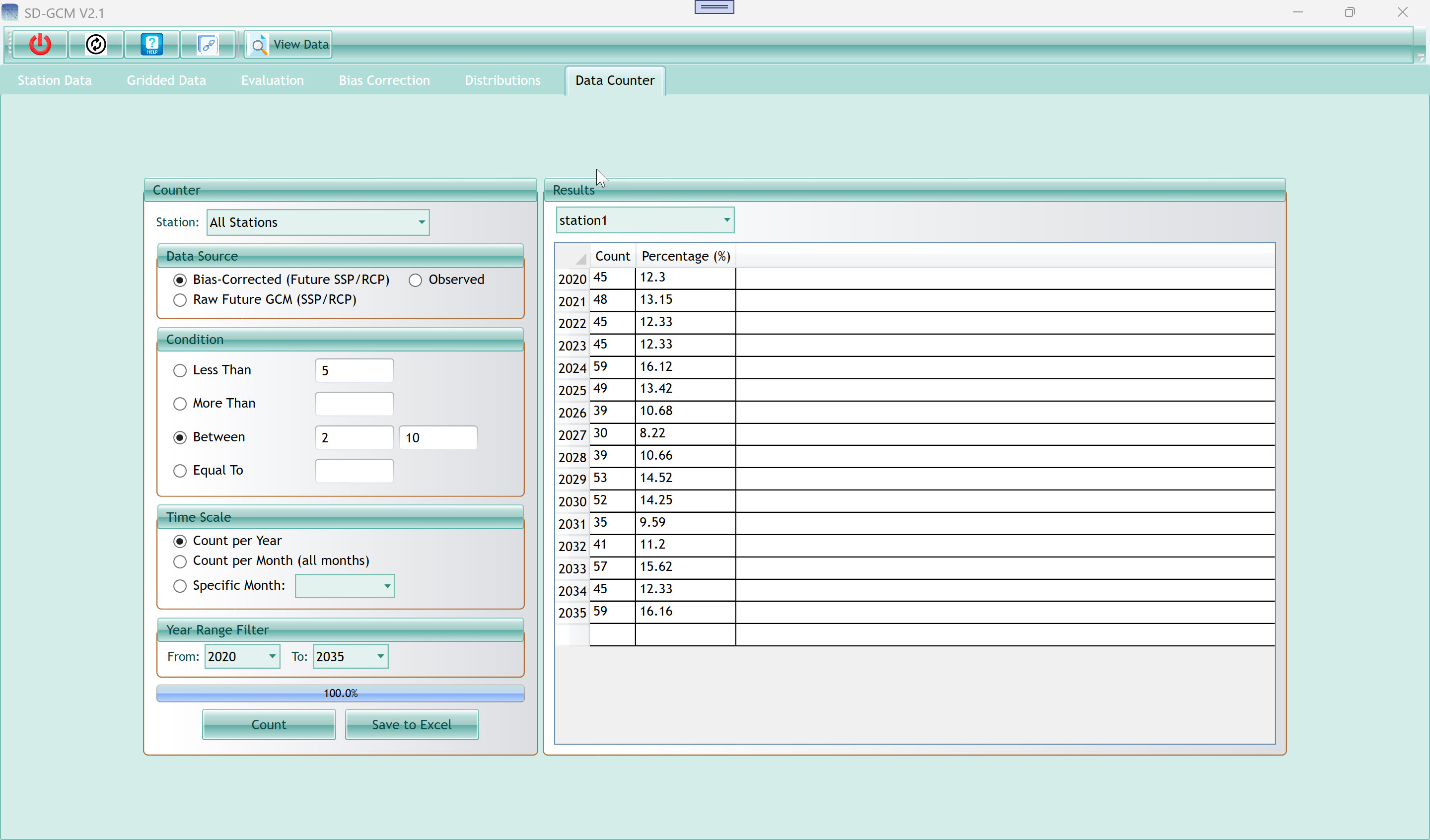
10. Data Counter Tab
The Data Counter tab counts how many time steps in any loaded dataset
satisfy a threshold condition, broken down by year or month. Common
uses: counting wet days (days with precipitation above a threshold),
counting extreme heat days (days above 35°C), counting drought days
(days with precipitation below 1 mm), or counting days within a range.
Results are shown both as raw counts and as percentages.
10.1 Counter Panel (Left)
10.1.1 Station Selector
| Station dropdown |
Select "All Stations" to count events for every loaded station
simultaneously (results are shown per station in the Results panel).
Select a specific station name to count only that station. "All
Stations" is the most common choice. |
10.1.2 Data Source
| Bias-Corrected (Future SSP/RCP) radio button |
Count events in the bias-corrected output from the Bias Correction
tab. Use this to quantify projected future changes in event
frequency. |
| Observed radio button |
Count events in the observed station data loaded in the Station Data
tab. Use this to characterise the historical baseline. |
| Raw Future GCM (SSP/RCP) radio button |
Count events in the raw (unit-converted but not bias-corrected)
future GCM data. Useful for comparing raw GCM vs bias-corrected event
counts. |
The Year Range Filter (below) automatically updates its year range to
match the selected data source — selecting Observed populates the filter
with observation years; selecting Future SSP/RCP shows the projection
years.
10.1.3 Condition
Select one condition and fill in the required value(s). Exactly one
radio button must be active.
| Less Than + value field |
Count time steps where the data value is strictly below the entered
number. Example: enter 1.0 to count days with precipitation below 1 mm
(near-dry days). |
| More Than + value field |
Count time steps where the value exceeds the threshold. Example:
enter 35.0 to count days above 35°C. |
| Between + two value fields |
Count time steps where the value falls in the range [value1, value2]
inclusive. Example: enter 2 and 10 to count days with precipitation
between 2 and 10 mm. |
| Equal To + value field |
Count time steps where the value exactly equals the entered number.
Most useful for counting exact zero-precipitation days (enter 0). Note
that floating-point values are compared with a very small tolerance
(10⁻⁹) to handle rounding. |
10.1.4 Time Scale
| Count per Year radio button |
Group results by calendar year. Each row in the Results table is one
year with a count and percentage for that year. |
| Count per Month (all months) radio button |
Group results by calendar month across all years. Each row is one
year, and each column is a calendar month (Jan–Dec). Results include
both count and percentage columns. |
| Specific Month radio button + dropdown |
Count only within a single selected calendar month. Choose the month
from the dropdown (January–December). Results are shown per year for
that month only. |
10.1.5 Year Range Filter
| From year dropdown |
Start year of the counting period. The dropdown is populated from
the selected data source's available years. Defaults to the first
available year. |
| To year dropdown |
End year of the counting period. Defaults to the last available
year. Restricting the range lets you count events in a specific future
decade or sub-period. |
| Progress bar (100.0%) |
Fills during computation. For large datasets with many stations,
this may take a few seconds. |
| Count button |
Run the counting analysis with the current settings. The Results
panel on the right updates immediately. |
| Save to Excel button |
Export the full Results table (all stations, all years/months, count
and percentage columns) to an Excel file. |
10.2 Results Panel (Right)
| Station selector dropdown |
After counting for All Stations, use this dropdown to switch between
stations in the results grid. Each station has its own results grid that
you can navigate independently. |
| Results grid |
Displays the counting results. Rows are years (or months within
years). Columns are Count (raw number of time steps satisfying the
condition) and Percentage (%) (count as a fraction of total time steps
in that year/month, expressed as a percentage). In the example shown,
2024 had 59 days with precipitation between 2 and 10 mm (16.12% of days
in 2024). |
Tip: To compare historical and future wet-day frequency, run the counter
twice: once with "Observed" selected (calibration years) and once with
"Bias-Corrected" selected (projection years). Save both and compare in
Excel.
The percentage column normalises for the fact that years have
different numbers of days when using a year range filter. It makes
inter-year and inter-station comparisons more meaningful than raw
counts.
For precipitation thresholds, a common set of indices from the ETCCDI
(Expert Team on Climate Change Detection and Indices): R10mm = days ≥ 10
mm; R20mm = days ≥ 20 mm; R1mm = days ≥ 1 mm (wet days). These can all
be computed with the "More Than" condition.
11. Complete Worked Example
This section walks through a full analysis from scratch using the
dataset visible in the screenshots: daily precipitation for two stations
(station1 at 35.19°N, 113.53°E and station2 at 34.48°N, 111.12°E) from
1993 to 2035.
Step 1 — Prepare your files
Observed station data: a CSV file with columns Date, station1,
station2 containing daily precipitation in mm, 1993-01-01 to 2012-12-31
(20 years).
Historical GCM file: a NetCDF file from MIROC6 historical
experiment covering 1993–2012, variable pr (precipitation flux, kg m⁻²
s⁻¹).
Future GCM file: a NetCDF file from MIROC6 SSP2-4.5 experiment
covering 2020–2035, variable pr.
Step 2 — Load the station
list
Open the Station Data tab.
In the "Fill Station List By File" panel, enter comma (,) as the
delimiter.
Click "Fill List by File" and select your station list
CSV.
In the GetData window, confirm First Row Is Header is checked,
set column assignments (Name of Station, Latitude, Longitude), and click
Load Data.
Verify the List Of Stations shows station1 (35.19, 113.53) and
station2 (34.48, 111.12).
Step 3 — Load observed data
In the "Load Data From File" panel, set delimiter to
comma.
Set Variable to "Rainfall".
Select "Daily data".
Leave Date format as "AutoDetect" (the dates are in M/D/YYYY
H:MM:SS AM format, which AutoDetect handles).
Click "Select Data File" and choose your observation
CSV.
In the column dropdowns at the top of the grid, assign: column 1
(Date) → Date; column 3 → station1; column 4 → station2.
Click "Load Station Data". The grid fills with daily
values.
Step 4 — Load GCM data
Switch to the Gridded Data tab.
Select Method 3 — NetCDF Files.
In Load Historical Data → Settings: click Select File and choose
the historical NetCDF. Set variable names: Time="time", Latitude="lat",
Longitude="lon". Set Time Units="days" and Since="1850-01-01". Set
Calendar="360_day" (check the file's metadata with ncdump -h).
In Load Historical Data → Loading: type "MIROC6" in GCM Model and
"historical" in Scenario. Select "pr" from the Variable
dropdown.
Click Load Historical. Wait for the progress bar to
complete.
Repeat the same steps for Load RCPs/SSPs Data using the SSP5-8.5
NetCDF file.
In the Unit Converter: select "Flux → mm/day" (converts kg m⁻²
s⁻¹ to mm/day). Set Correction Factor to Multiplicative. Click Save
Settings.
Step 5 — Evaluate methods
Switch to the Evaluation tab.
Set Observation Period to 1993–2012, Historical GCM Period to
1993–2002, Evaluation Period to 2003–2012.
For each of the six methods (and optionally with Monthly
Stratification checked), click Evaluate then Add to Comparison.
Review the Method Comparison table. Look for the row with the
best KGE and NSE on the 2003–2012 evaluation period.
In this example, SDM_M (SDM with Monthly Stratification) shows
KGE=0.575, NSE=0.196, WDF=1.047 on the evaluation period — a good result
for daily precipitation.
Click Save Results to export the comparison table.
Step 6 — Apply bias
correction
Switch to the Bias Correction tab.
Set Station Period to 1993–2012, Historical Period to 1993–2012,
Downscale Period to 2020–2035.
Select SDM, check Monthly Stratification.
Click Downscale. The chart shows the corrected projection (green)
against the raw GCM (red dashed) and observed (blue).
Check the Time Series chart: the green corrected series should
show more rainfall amplitude than the raw GCM near-zero values.
Click Save DownScaled Data to export the final corrected daily
time series.
Step 7 — Analyse the output
Switch to the Distributions tab. Set Use Monthly Data and Use
Downscaled Data. Click Check 12 Distributions for station1.
In the Distribution Fitting window, identify the best-fitting
distribution from the Rankings tab (lowest AD statistic that is not
999).
Switch to the Data Counter tab. Select Bias-Corrected, Between
condition with values 2 and 10, Count per Year, years
2020–2035.
Click Count. Review how the number of moderate-rainfall days
changes across the projection period.
Click Save to Excel to record the results.
12. Common Issues and Tips
12.1 Units Mismatch
Symptom: NSE is very negative (−10 or worse), the corrected time
series is orders of magnitude off from the observed.
Cause: the Unit Converter was not set or was set incorrectly.
Fix: return to the Gridded Data tab, check the raw GCM values in View
DB (e.g. if daily precipitation shows values around 0.0001, it is in kg
m⁻² s⁻¹ and needs ×86400). Set the correct conversion and click Save
Settings, then re-run Evaluation.
12.2 Dates Not Parsing
Correctly
Symptom: date column shows wrong years, or evaluation period
dropdowns are populated with unexpected values.
Cause: AutoDetect selected the wrong date format, or your Excel file
stores years as numeric integers (e.g. 1993.0).
Fix: in the Station Data tab, change the Date format dropdown from
AutoDetect to the explicit format that matches your file (e.g. "yyyy"
for year-only columns). The tool handles the integer-to-date conversion
automatically when a format is explicitly specified.
12.3 CDS Download Fails with
HTTP 403
Cause: you have not accepted the CMIP6 Terms of Use on the CDS
website.
Fix: log into cds.climate.copernicus.eu, search for "CMIP6 climate
projections", open the Download Data tab, scroll to the bottom, and
accept the licence. Then retry.
12.4 CDS Download Fails with
HTTP 401
Cause: the API key is wrong, expired, or in the old UID:APIKEY
format.
Fix: go to cds.climate.copernicus.eu/profile and copy your current
Personal Access Token. It is a plain UUID with no colon. Paste it into
the API Key field and click Save key.
12.5 Distribution
Fitting Shows All Rank 999
Cause: data contains NaN, Inf, negative values, or zeros that prevent
distribution fitting.
Fix: in the Distributions tab, check "Remove Values Less Than" and
set the threshold to 0 (or a small positive number like 0.1 for
precipitation). Then click Check 12 Distributions again.
12.6 KGE and NSE Are Poor on
Evaluation
This is a sign of overfitting — the transfer function has memorised
the calibration data rather than learning a generalisable correction. It
is especially common when Monthly Stratification is used with short
calibration periods (fewer than 10 years per month = fewer than 1 year
per month).
Fix: either use a longer calibration period, or use the
non-stratified version of the same method (e.g. switch from QDM_M to
QDM).
12.7 Scientific
Guidance: Which Method to Choose?
For temperature: EQM_M or QDM_M. EQM_M is sufficient for most
temperature applications. QDM_M is preferred if the study focuses on
extreme heat events, since it preserves the warming signal at every
quantile of the distribution.
For precipitation: SDM_M or QDM_M. SDM_M explicitly corrects
wet-day frequency (drizzle bias) and is recommended as the default.
QDM_M is preferred when the study needs to preserve projected changes in
heavy precipitation extremes.
For wind speed or humidity with small bias: Delta_M is often
adequate and produces the most interpretable correction (a simple
seasonal scaling factor).
Rule of thumb: if your Evaluation tab results show that a method
performs well on the calibration period (same period rows) but poorly on
the evaluation period (separate period rows), prefer the method with the
smallest degradation between periods, not the one with the highest
same-period score.
https://agrimetsoft.com/sd-gcm |
https://www.youtube.com/AgriMetSoft
For support, video tutorials, and additional documentation visit our
website.
Open PDF
Download PDF
Formulas →
Back to SD-GCM