Open PDF
Download PDF
OSF mirror
Formulas →
Back to IDF Curve
This tutorial walks you through using the IDF Curve tool to construct
rainfall Intensity-Duration-Frequency (IDF) curves from your data. It
covers the original workflow and the new capabilities added in the
latest update: water-year support, incomplete-year handling, the
Generalize Extreme Value (GEV) and Log-Pearson Type III (LP3)
distributions, the Goodness-of-Fit table, 90% confidence bands, the IDF
Equation dialog with Sherman and Koutsoyiannis fitting, custom return
periods, and several smaller refinements.
Each major new feature is marked with a "New in this update" callout
so you can scan for the additions if you already know the previous
version.
1. License and Installation
Installing the tool is straightforward. Once you purchase a license,
you will receive a small utility called "ID Finder." After sending us
the ID, you will receive the installer for the registered version.
Simply run the installer, and the tool will be installed and ready for
use without the need for a key. After installation, you can access the
tool either by clicking on the desktop shortcut or by searching for "IDF
Curve" in your computer’s program list.
The tool accepts data in two ways:
Raw rainfall time series (Input Raw Data tab). The tool will
compute maxima for each duration and build a Rainfall Intensity Table
for you. This is the most common workflow.
Precomputed Rainfall Intensity Table (Input Data tab). If you
already have a table of maximum intensities per duration per year, you
can load it directly and skip the maxima computation.
2.1 Loading raw data
Gather historical rainfall data for the location of interest. You can
obtain this data from government meteorological agencies, research
institutions, or local weather stations. Online databases and climate
archives are valuable resources.
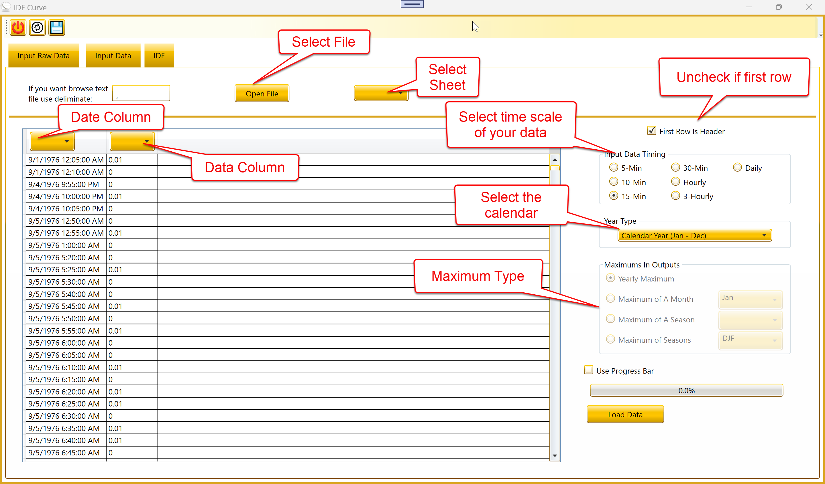
On the Input Raw Data tab:
Click Open File and select your Excel workbook.
Choose the worksheet that contains the data.
Make sure your date column is formatted as Excel Date.
Set the time scale of the input data correctly — 5 minute, 10
minute, 15 minute, 30 minute, hourly, etc. Choosing hourly when your
data is actually in 3 hour intervals will produce incorrect
calculations.
Click Load Data.
If your record has gaps, the tool will offer to fill them. You can
choose your fill method per gap; the "Do it for all items" option
applies the same method to every remaining gap.
2.2 Year Type and Maximums in
Output
The tool now supports any starting month for the year, including
water-year conventions used in hydrology.
The default year type is the calendar year (January to December), but
you can pick any month as the year start. The most common alternative is
the water year, which in the United States Geological Survey convention
runs from October to September and is labeled by the year in which it
ends. So water year 2025 covers October 2024 through September 2025.
Why this matters: rainfall seasonality often crosses the calendar
boundary. A wet season that spans November to March is split into two
different calendar years, which weakens the yearly maximum statistics.
Using a year type aligned with the local seasonality keeps each season
inside a single year.
Under "Maximums in Output," you can choose:
Yearly Maximum — the annual maximum series (AMS), the most common
choice for IDF analysis.
Maximum for a Specific Month — useful for monsoon studies and
other strongly seasonal climates.
Maximum for a Predefined Season — see the table of twelve seasons
in the Reference section below.
Custom Months — pick any set of months (e.g., February, March,
April, June, July).
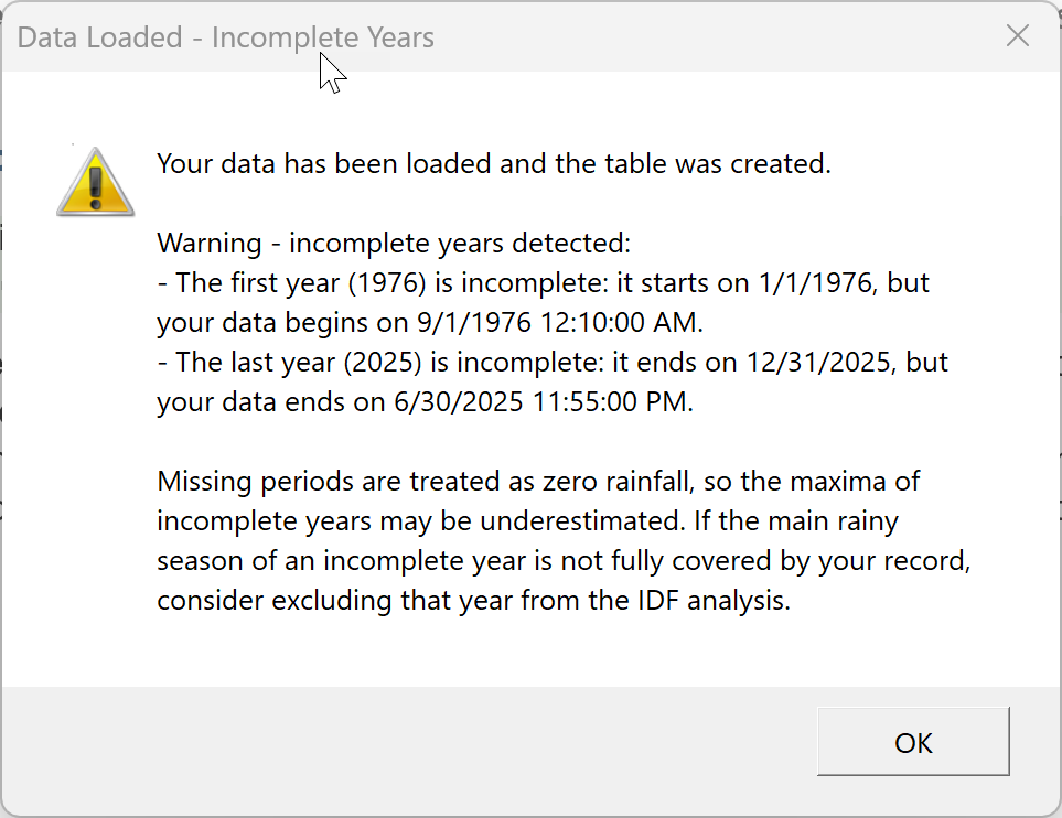
2.3 Incomplete Years Warning
The tool detects partial first or last years in the record and offers
to exclude them from the distribution fit.
After loading raw data, the tool checks whether the first and last
years of the record are complete according to the chosen year type. If
they are not, a warning dialog lists the partial years.
Example: with a water year starting in October and a record from
September 1976 to June 2025, both the first water year (1976: October
1975 through September 1976, missing October 1975 to August 1976) and
the last water year (2025: October 2024 through September 2025, missing
July to September 2025) are incomplete.
Incomplete years bias the maxima downward, because missing periods
are effectively treated as zero rainfall. Including them in the fit can
pull the IDF curves below their correct level, especially at long return
periods.
On the IDF tab there is a checkbox labeled "Exclude incomplete
years." When the tool detects partial years in the record, this checkbox
is automatically ticked and the partial years are excluded from the
distribution fit. You can untick it if you specifically want to include
them, but ticking it is the safer default.
3. The IDF Tab
3.1 Return Periods
(editable)
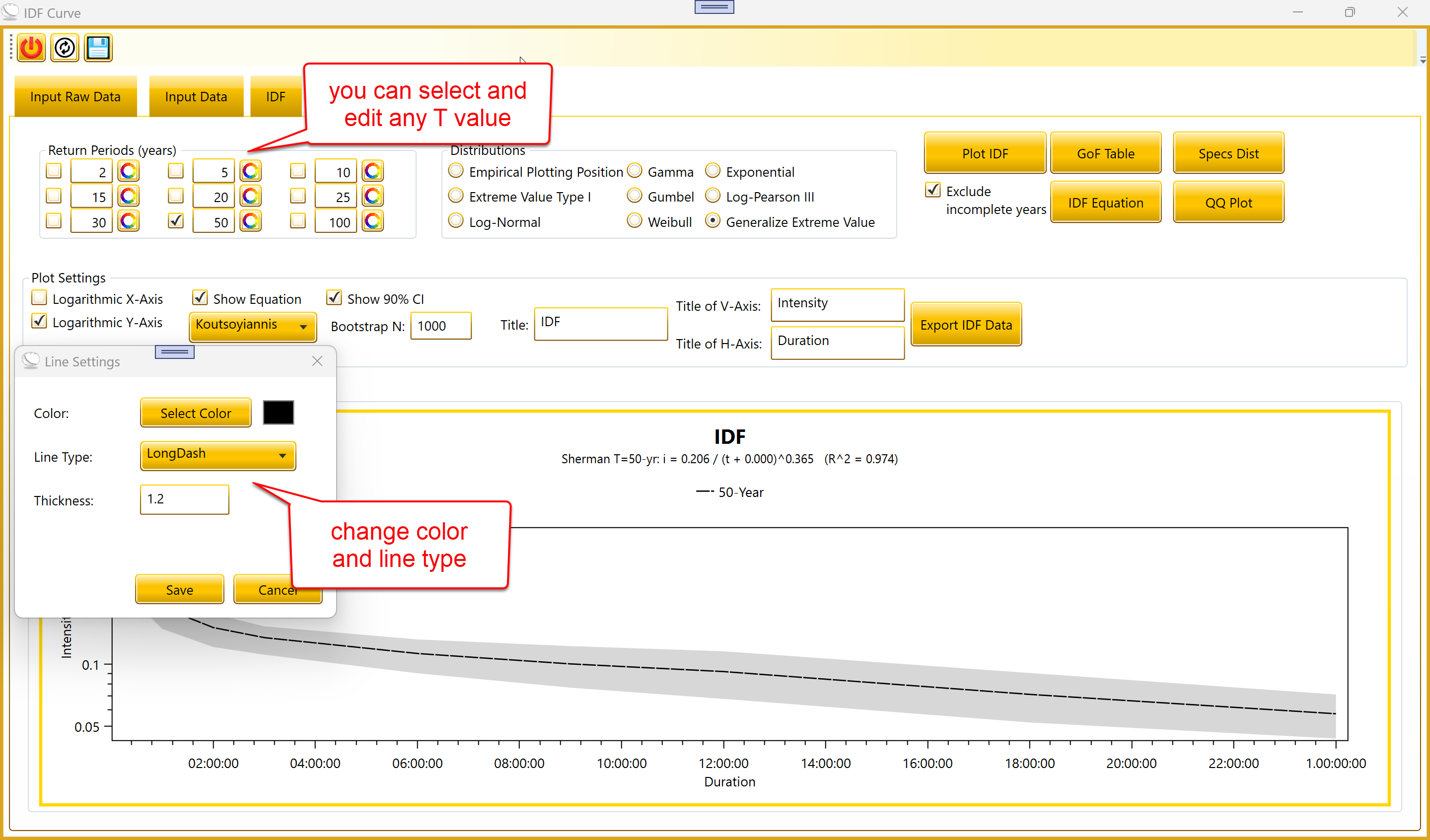
Each return-period checkbox now has an editable number next to it.
You can type any T value, including 200, 500, or 1000.
Nine checkboxes select which return periods to include in the plot.
Each has an adjacent editable text field with the T value in years.
Default values are 2, 5, 10, 15, 20, 25, 30, 50, and 100. You can change
any number to a custom value by typing into the textbox. When you click
Plot IDF, the tool computes quantiles for whichever T values are
currently checked.
A small color/style button next to each row opens the Line Settings
dialog. You can choose the line color, dash style, and thickness used to
draw that T’s curve on the plot.
When you click Plot IDF, if any selected T is greater than 2x the
record length (in years), a warning lists the affected return periods.
For a 48-year record, asking for 100-year quantiles is reasonable, but
asking for 500-year or 1000-year quantiles is heavy extrapolation — the
fitted distribution is being asked to predict events far beyond what
your data has constrained.
The values are still computed, but they should be interpreted with
caution and reviewed before any design use. The Excel export and the IDF
Equation CSV both annotate the affected return periods.
3.2 Distributions
Two new distributions are available: Generalize Extreme Value (GEV)
and Log-Pearson Type III (LP3). Both use methods that match
international hydrology standards.
The tool supports seven probability distributions for frequency
analysis:
| Empirical Plotting Position (EPP) |
0 (non-parametric) |
Weibull plotting positions p = i / (n + 1) |
Quick visual check; cannot extrapolate beyond ~n years |
| Extreme Value Type I (Gumbel) |
2 |
Method of moments (mean, std) |
Classical extreme-value fit; assumes light upper tail |
| Gamma |
2 |
Maximum likelihood (Accord) |
Common for daily precipitation totals |
| Exponential |
1 |
Maximum likelihood (Accord) |
Simple single-parameter form |
| Log-Normal |
2 |
Maximum likelihood (Accord) |
Empirically good for rain amounts |
| Weibull |
2 |
Maximum likelihood |
Flexible shape for time-to-event data |
| Generalize Extreme Value (GEV) |
3 |
L-moments (Hosking 1990) + Newton refinement |
Recommended for AMS; covers Gumbel as limit |
| Log-Pearson Type III (LP3) |
3 |
Bulletin 17B (log-skewness + Kite factor) |
U.S. standard for flood frequency analysis |
The detailed mathematical formulation of each distribution is in the
companion Formulas document. The choice of distribution affects every
output: the IDF curves, the confidence bands, the IDF Equation
coefficients, and the goodness-of-fit ranking.
3.3 Plot Settings
Click Plot IDF to compute and draw the curves. Several plot-settings
options affect how the result is displayed:
Logarithmic X-Axis / Logarithmic Y-Axis — switch each axis to log
scale. The logarithmic horizontal axis displays values as log10(time) in
seconds.
Show 90% CI — adds shaded bootstrap confidence bands around each
curve. See the next section.
Bootstrap N — the number of bootstrap resamples used for the
bands. 1000 is the standard choice; 500 is faster; 2000 is smoother.
Only used when "Show 90% CI" is ticked.
Show Equation — adds the fitted IDF equation as a subtitle on the
plot. The dropdown next to it picks which form to show: Koutsoyiannis
(global) or Sherman (at the median selected T).
Title, Title of V-Axis, Title of H-Axis — text labels for the
plot. These also propagate to the Excel chart on export.
3.4 90% Confidence Bands
Shaded bands around each return-period curve, computed by bootstrap
resampling.
When "Show 90% CI" is ticked, the tool computes 90% bootstrap
confidence bands around each return-period curve. The bands are obtained
by resampling the annual maxima with replacement (Bootstrap N times),
refitting the chosen distribution to each resample, and taking the 5th
and 95th percentiles of the resulting quantile distribution at each
duration.
The bands show the range where the true population quantile likely
lies, given the limited sample size. They are not predictive intervals
for an individual storm; the actual rainfall in any given year can lie
outside the band.
Note: If the fitted line falls outside its own band,
that points to either a poor distributional choice or an estimator
inconsistency. The latest version of the tool uses a single Gumbel
estimator (Accord maximum likelihood) for the line, the band, the GoF
Table, and the Specs Dist dialog, so the line should sit inside the band
for Gumbel on most records. For non-Gumbel data the line can still be
far from the empirical points; that is a fit-quality issue, addressed by
switching to GEV or LP3.
3.5 IDF Equation
Fit closed-form IDF equations to your curves and export the
coefficients to CSV.
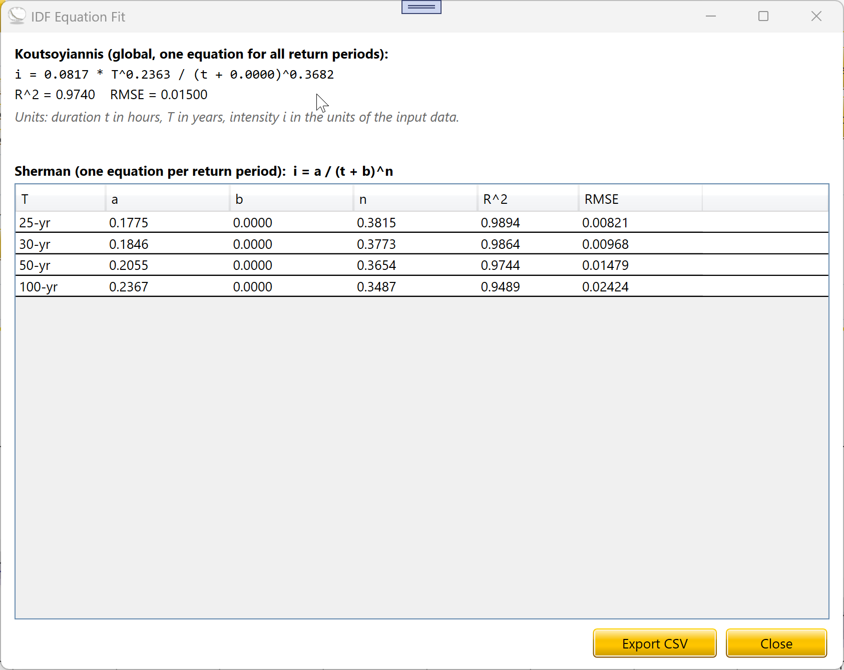
The IDF Equation button fits closed-form intensity equations to the
plotted curves. Two equation forms are produced together:
Sherman (per return period): i = a / (t + b)^n. One fit per
selected T. The coefficients a, b, n vary with T.
Koutsoyiannis (global): i = a · T^m / (t + b)^n. A single fit
covering all selected return periods together. The coefficients a, m, b,
n are constants across the entire IDF surface.
The dialog shows both fits side by side, including R² and RMSE for
each. Sherman’s per-T table can be reviewed row by row. The
Koutsoyiannis equation is shown in the dialog header in human-readable
form.
The Export CSV button saves both fits to a plain-text file. Units are
duration t in hours, return period T in years, and intensity i in the
units of your input data. If any selected return period was flagged as
extrapolation, the CSV includes a warning comment at the top naming the
affected T values, so reviewers can see immediately which numbers are
heavy extrapolations.
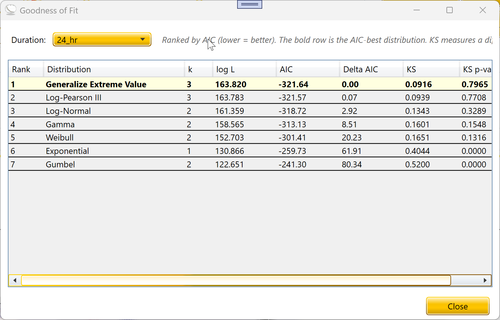
3.6 Goodness-of-Fit Table
Compare all seven distributions on the data for the selected
duration. Ranked by AIC; the AIC-best row is highlighted.
The GoF Table button compares all seven distributions on the data for
the selected duration. The table shows, for each distribution:
k — number of parameters
log L — log-likelihood (higher is better)
AIC — Akaike Information Criterion (lower is better; balances fit
against complexity)
Delta AIC — difference from the best distribution’s AIC
KS — Kolmogorov-Smirnov statistic, the largest gap between fitted
and empirical CDF (smaller is better)
KS p-value — using Stephens (1970) finite-n correction; the same
formula Accord’s KolmogorovSmirnovTest uses internally
The table is sorted by AIC, smallest first. The top row is shown in
bold with a light-yellow background — this is the AIC-best distribution.
KS measures a different aspect of fit (the worst-point gap between
fitted and empirical CDFs) and may rank distributions slightly
differently from AIC. A common rule of thumb is that Delta AIC < 2
indicates two distributions are essentially tied; Delta AIC > 10
indicates the lower-AIC distribution is clearly preferred.
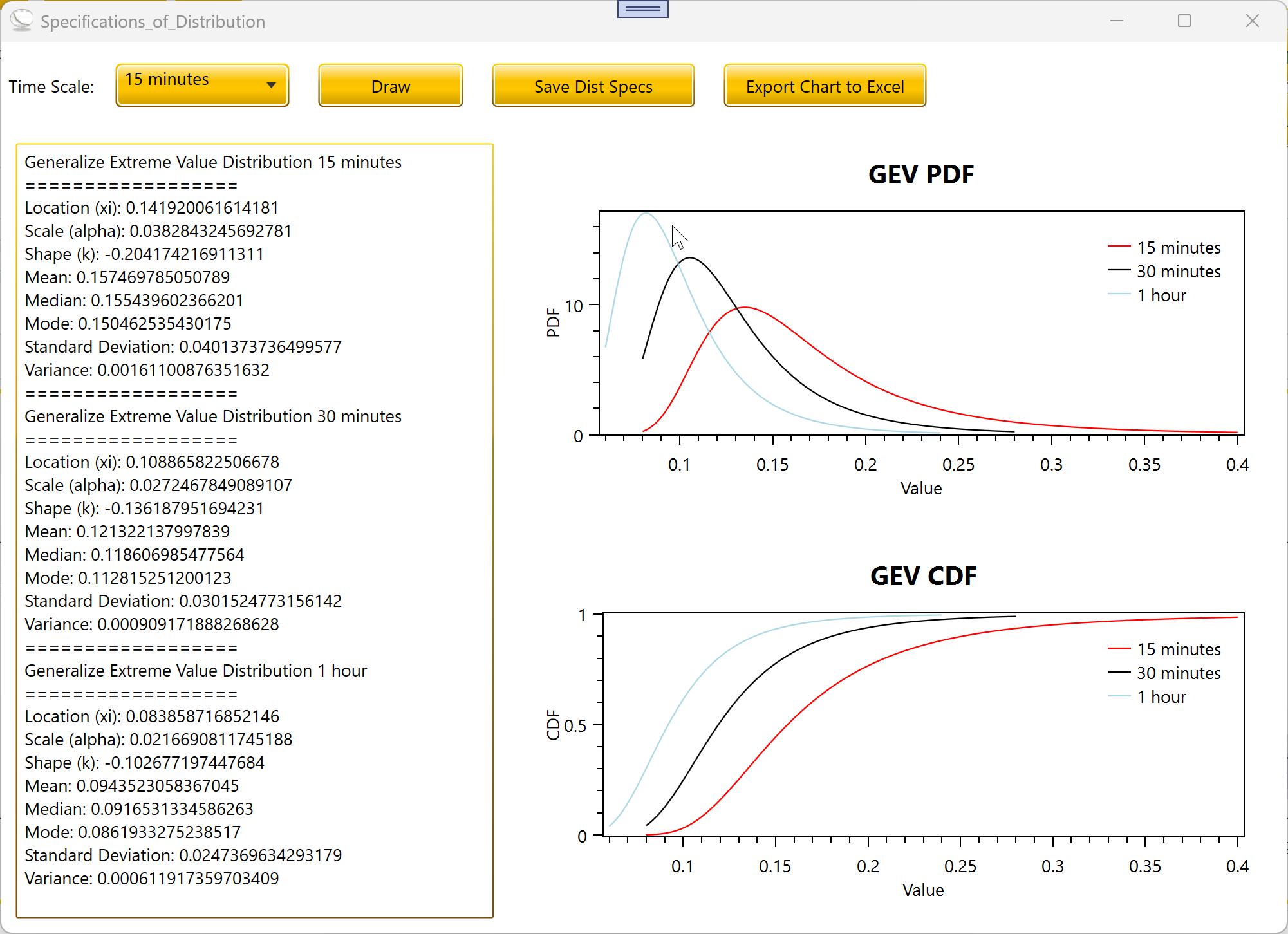
3.7 Specifications of
Distribution
Specs Dist now supports GEV and LP3 in addition to the Accord-backed
distributions.
The Specs Dist button opens a window with the fitted parameters and
analytical properties of the currently selected distribution at the
chosen duration. For all seven distributions including GEV and
Log-Pearson III, it shows:
The fitted parameters (e.g., for GEV: location xi, scale alpha,
shape k; for LP3: log-mean mu, log-std sigma, log-skew g).
Mean, median, mode, standard deviation, and variance, where these
are defined for the fitted parameter values.
CDF and PDF curves over the data range.
For GEV, certain moments are only defined for certain ranges of the
shape parameter: the mean exists when k < 1, the variance exists when
k < 0.5, and the mode exists when k > -1. The dialog explicitly
flags these as undefined when they cannot be computed for the fitted
shape.
For Log-Pearson III, the reported parameters (mu, sigma, g) are on
the log10 scale. The median in real space is reported separately,
computed using the Kite frequency factor at p = 0.5.
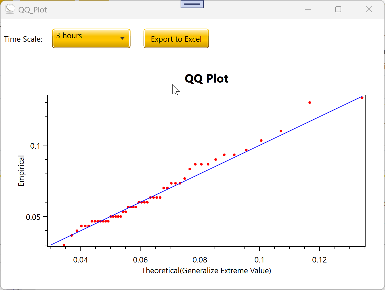
3.8 Q-Q Plot
Q-Q Plot now supports GEV and Log-Pearson III in addition to Gamma,
Log-Normal, Exponential, Weibull, and Gumbel.
The Q-Q Plot button shows a Q-Q diagnostic — theoretical quantiles on
the X axis against empirical quantiles on the Y axis. A good fit
produces points close to the 1:1 diagonal reference line.
For GEV and LP3, the dialog re-fits the distribution from the same
data the IDF curves used, so the Q-Q diagnostic exactly mirrors the fit
shown on the plot. Points along the diagonal in the body of the
distribution with a small deviation at the highest ranks is normal —
that is what a heavy upper tail or an outlier looks like, and it is
information about the data, not a tool bug.
3.9 Line Settings
The Line Settings dialog has been rewritten. The previous version
could carry over selections between dialog sessions; the new version
applies your changes only when you click Save, and a Cancel never
modifies the line.
Clicking the small color button next to a return-period checkbox
opens the Line Settings dialog. You can pick:
Color, via the standard Windows color picker.
Line type, including Solid, Dash, Dot, DashDot, and several other
patterns.
Thickness, as a decimal number (default 1.2).
A small swatch next to the Select Color button shows the chosen color
before saving. The Save and Cancel buttons respond to Enter and Escape
respectively.
4. Exports
4.1 PNG image
The save icon in the top bar saves the current IDF plot as a PNG
image at the on-screen resolution.
4.2 Excel IDF Data
When the 90% CI is enabled, the Excel export now includes Low / Mid /
High columns for each return period.
The Export IDF Data button in Plot Settings opens Excel with the full
IDF table and a default chart. The first column is Duration; each
selected return period gets its own column. If "Show 90% CI" was ticked
when you last clicked Plot IDF, each return period gets three columns
labeled (Lo), main value, and (Hi), so the band data travels with the
table.
The Excel chart plots the main lines only by default; the band
columns are present in the spreadsheet so you can add them to the chart
yourself if you want a visual band. The chart axis titles match the
"Title of V-Axis" and "Title of H-Axis" fields from Plot Settings.
4.3 CSV Equation Coefficients
Coefficients export from the IDF Equation dialog.
In the IDF Equation dialog, the Export CSV button saves both the
Koutsoyiannis and Sherman fits to a comma-separated file. The format
includes commented header lines (starting with #) explaining units. The
file is plain text and works in any spreadsheet program or analysis
script.
Units in the file: duration t is in hours, return period T is in
years, and intensity i is in the units of your input data. The CSV also
includes a warning block at the top if any selected T was flagged as
extrapolation.
5. Warnings and Limitations
This section consolidates the cautions noted earlier so they are easy
to find.
Warning: EPP is a non-parametric method. It
estimates quantiles at empirical plotting positions, which means it
cannot produce a value for any return period larger than approximately
the sample size.
If you select EPP and a return period that is too large (for example,
T = 200 years with a 48-year record), the tool returns invalid values
for those columns and a specific warning will appear. The IDF Equation
dialog automatically skips those rows. For T values beyond the sample
size, you must use a parametric distribution such as GEV, LP3, or
Gumbel.
Warning: For parametric distributions, quantiles for
T values larger than approximately 2x your record length are heavy
extrapolations of the fitted distribution.
The numbers are mathematically defined but their accuracy depends
entirely on whether the fitted distribution correctly describes the
upper tail — something a short record cannot verify. Use these values
with caution, and prefer GEV or LP3 over Gumbel for upper-tail
estimates. The Excel export and the IDF Equation CSV both annotate the
affected return periods so reviewers are alerted.
5.3 Confidence
bands are statistical, not predictive
Warning: The 90% bootstrap bands describe
uncertainty in the fitted quantile due to limited sample size; they do
not predict the range of actual rainfall amounts.
An individual year’s rainfall can lie well outside the band even when
the fit is correct. For predictive intervals on a specific storm, a
different methodology is required.
5.4 Incomplete years bias
maxima downward
Warning: A partial year contains fewer rainfall
observations than a complete year, so its maximum is on average smaller.
Including partial years in the AMS pulls the fitted distribution
downward.
The "Exclude Incomplete Years" checkbox handles this; we recommend
leaving it ticked when the tool has detected partial years. Untick it
only when you have verified that the partial year does in fact contain
the annual maximum.
5.5 Goodness-of-Fit
p-values are for ranking
Warning: When the distribution is fitted from the
same sample being tested, the Kolmogorov-Smirnov p-value is
conservatively high — it does not penalize the fact that the parameters
were estimated from the data. This is a known property of the test, not
specific to this tool.
The values shown in the GoF Table are appropriate for ranking
distributions against one another, which is what the table is designed
for. For formal hypothesis testing on a specific distribution, use
Anderson-Darling or a bootstrap KS test instead.
6. Reference: Twelve
Predefined Seasons
The seasonal maxima option groups months into rolling three-month
windows. Each season is labeled by the initials of its three months.
| DJF |
December, January, February (Winter) |
| JFM |
January, February, March (Winter to Spring transition) |
| FMA |
February, March, April (Early Spring) |
| MAM |
March, April, May (Spring) |
| AMJ |
April, May, June (Late Spring) |
| MJJ |
May, June, July (Early Summer) |
| JJA |
June, July, August (Summer) |
| JAS |
July, August, September (Summer to Autumn transition) |
| ASO |
August, September, October (Early Autumn) |
| SON |
September, October, November (Autumn) |
| OND |
October, November, December (Late Autumn) |
| NDJ |
November, December, January (Autumn to Winter transition) |
7. Further Resources
Tool website: https://agrimetsoft.com/idf_curve
Tutorial videos and channel: http://www.youtube.com/AgriMetSoft
For the mathematical details of each distribution, the bootstrap
procedure, the goodness-of-fit metrics, and the IDF equation fitting
algorithm, see the companion document "Formulas.docx".
Open PDF
Download PDF
OSF mirror
Formulas →
Back to IDF Curve